Received 8 June 2015; accepted 13 November 2015; published 16 November 2015

ABSTRACT

We present a class of axially symmetric and stationary spaces foliated by a congruence of surfaces of revolution. The class of solutions considered is that of Carter’s family [A] of spaces and we try to find a solution to Einstein’s equations in the presence of a perfect fluid with heat flux. This approach is an attempt to find an interior solution that could be matched to a corresponding exterior solution across a surface of zero hydrostatic pressure. The presence of a congruence of surfaces of revolution, described as the quotient space of the commoving observers, can be useful to the determination of the surface of zero pressure. Finally we present two formal solutions representing ellipsoids of revolutions.

Keywords:

General Relativity, Exact Solutions

1. Introduction

The contents of this paper summarize and improve a series of papers in which I have tried to solve the problem of constructing an interior Kerr solution, [1] - [4] . By this we mean the search for a material body that could generate a vacuum field described by the Kerr solution. This search still remains without results after more than 53 years of its discovery. The corresponding problem in the Newtonian theory of gravitation, in the case of homogeneous density distribution has been found satisfactory solutions, with contributions of some of the greatest scientists: Newton, Jacobi, Dedekind, Dirichlet, Riemann, Poincare, H. Cartan, and others [5] . The problem in the context of the General Theory of Relativity can be set as follows: Find all possible equilibrium configurations, satisfying, Einstein’s equations, bounded by a surface of zero hydrostatic pressure, matched across this surface, to a vacuum solution, sharing the same symmetries (stationarity and axial symmetry); see Geroch and Lindblom [6] . A very detailed review of the many different attempts to solve this problem can be found in a paper of Krasinski [7] . He gave a perspective of solution, by analogy to the Newtonian theory, in which the surface of the rotating body was an ellipsoid of revolution. He defined the notion of confocal ellipsoids in the curved spaces of General Relativity. Unfortunately he has not found any new interior solution and his approach was not pursued further. The same problem is also mentioned in [8] with very interesting commends. After a long period of time, Racz [9] considered stationary and axially symmetric vacuum spaces, possessing a one parameter congruence of confocal ellipsoids, generalizing the work of Krasinski. In the same spirit Zsigrai [10] generalized the definition of an ellipsoid in curved spaces and presented as example stationary and axially symmetric perfect fluid solutions with the so called confocal inside ellipsoidal symmetry. Our approach is based on a generalization for the bounding surface of the fluid: we are searching for the most general surface compatible with the assumption of axial symmetry. The most general family of surfaces compatible with the axial symmetry is that of surfaces of revolution. Namely, the surfaces obtained by revolving a plane curve C, about a line L, belonging to its plane and identifying the line L to the axis of rotation of the interior configuration. The next step is to consider the Einstein’s equations inside and outside the surface of revolution. The first part of this paper concerns the construction of a foliation, for the stationary and axially symmetric spaces of General Relativity, by a congruence of surfaces of revolution. Then we are searching for solution of Einstein’s equations in the Carter’s family [A] of spaces compatible with the above mentioned foliation. Carter’s family of spaces is a case of stationary and axially symmetric solutions and it contains the Kerr-NUT solution and many other interior solutions; see [11] - [15] . In Section 2, we give a brief description of Carter’s family [A] of spaces. In Section 3 we define the metric tensor of a 3-dimensional Riemannian space representing a congruence of surfaces of revolution. This definition permits to obtain the corresponding 4-dimensional Lorentzian space, whose quotient space with respect a class of observers is identifying with the above defined 3-dimensional Riemannian space. In Section 4 we write explicitly the Einstein’s equations for Carter’s family [A] of spaces, admitting a foliation by the surfaces of revolution (ellipsoids or tori). Finally in Section 5 we present two solutions admitting the above mentioned foliation by confocal ellipsoids.

2. Carter’s Family [A] of Spaces

We suppose that the space-time admits an Abelian isometry group G₂, invertible with non-null surface of transitivity [11] , then the metric tensor can be written as follows:

(2.1)

The components of the metric tensor (2.1) depend on x and y, the G₂ group is generated by the time-like Kill-

ing field (implying the stationarity) and the space-like Killing field (implying the axial symmetry).

The invertibility of the group is obvious from the fact that the transformation is an isometry. The metric (2.1) can be put in a more convenient for calculations form, the symmetric tetrad form, in which the Newman-Penrose (NP) coefficients are equal by pairs:

(2.2)

The functions L, M, N, P are real and depend only on x and y. This metric has been introduced by Carter and used extensively by Debever [11] Carter and McLenaghan [13] and by us [14] , [15] . The Einstein’s equations for the metric (2.1) even in the case of vacuum are very complicated so we restrict our study to the Carter’s family [A] of spaces:

(2.3)

This family of spaces is characterized by the fact that the Hamilton-Jacobi equation for the geodesics is solvable by separation of variables (x, y), which takes place in a particular way and gives rise to a fourth constant of motion, quadratic in the velocities integral or equivalently to the existence of a Killing tensor with two double eigenvalues, see [16] and references cited there. In the NP formalism and in the context of complex vectorial formalism of Cahen, Debever, Defrise, this Killing tensor can be written as follows:

(2.4)

The metric is:

where:

(2.5)

The null vectors n, l are real and, are complex conjugate. The notation of the formalism can be found in [17] , [18] , and [19] .With an appropriate choice of the null tetrad (2.5), the components the Weyl tensor and the Ricci traceless tensor in the NP formalism satisfy the following relations:

(2.6)

The Carter’s family [A] of solutions includes many interesting metrics, we present some of them in order to make easier the comparison with our solution and justify some technical details of calculations.

2.1. Kerr-NUT Solution with or without Cosmological Constant [Metric (17) in [11] )

The Einstein’s vacuum equations imply that:

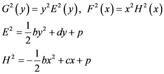(2.7)

where b, c, d, p are constants of integration. The Kerr metric is obtained if we set:

(2.8)

(2.9)

m is the mass, a is the parameter of angular momentum per unit mass and the Kerr metric can be written in the Boyer-Lindquist coordinates:

(2.10)

,

2.2. Wahlquist Solution

The Einstein’s equations in the presence of a perfect fluid reduce to two relations:

(2.11)

(2.12)

These equations ensure that the energy-momentum tensor admits one simple and one triple eigenvalues. The solution of (2.11) permits us to determine the following functions:

(2.13)

where are constants of integration and by defining new coordinates:

(2.14)

We get Wahlquist solution [15] , [20] (and are the Wahlquist coordinates).

3. Stationary and Axially Symmetric Spaces Foliated by a Congruence of Surfaces of Revolution

We consider a 3-dimensional Euclidean space foliated by a congruence of surfaces of revolution, obtained by revolving a plane curve C about a line L in its plane. This line will be identified with the axis of rotation of the fluid configuration. In a Cartesian coordinate system the curve C belongs to the plane and the axis of rotation. In this coordinate system a parametric representation of the curve C, is given by:

(3.1)

where t is the corresponding parameter. The elimination of this parameter between x₁, x₃ gives the Cartesian equation of the curve:

(3.2)

The Cartesian equation of the surface is:

(3.3)

Then a parametric representation of a surface of revolution is:

(3.4)

We can now define a system of coordinates, adapted to the surface of revolution. The azimuthal angle measured around the axis of rotation, is one of them, the other two being r and some kind of generalized spherical coordinates related by an equation which is precisely the equation of the surface of revolution. Then (3.4) can be put in the following form:

(3.5)

And the equation for each member of the congruence of the surfaces of revolution is given by:

(3.6)

The corresponding metric in the Euclidean space assumes the expression:

(3.7)

where,

The coordinates are orthogonal if:

(3.8)

We will consider only orthogonal coordinate systems and we generalize (3.7) to a three-dimensional axisymmetric Riemannian space by considering a supplementary function:

(3.9)

Obviously when we get the corresponding Euclidean metric (3.7). This generalization is useful because it keeps the factor h₁ containing the parametric representation of the curve C.

Finally we introduce a coordinate change of great utility for the integration of Einstein’s equations. Instead of r and θ we will use y and x that appear in (2.3). This coordinate transformation is given by (2.9), the coordinate used to obtain Kerr metric from the Carter’s family [A] of spaces.

Definition 3.1.

The metric of a three-dimensional Riemannian space foliated by a congruence of surfaces of revolution, in an orthogonal coordinate system is given by:

(3.10)

And the orthogonality condition holds:

(3.11)

The observers who will describe the shape of the two-dimensional surfaces embedded in the four-dimensional Lorentzian space as rotating surfaces of revolution (defining the equipotential or equipressure surfaces for the vacuum and the interior case respectively), follow the trajectories of the symmetry group. The velocity field of

this family of observers is then a linear combination of the Killing vector fields.

Definition 3.2.

The vector field of the family of the observers describing the surfaces of revolution is given by:

(3.12)

And as usual the norm is given by:

(3.13)

where are the metric coefficients of (2.2).

The observers defined above are at rest on their quotient space that has to be identified with the three-dimen- sional Riemannian space of the Definition (3.1):

(3.14)

This equation and the relations (3.12), (3.13) imply the following conditions:

(3.15a)

(3.15b)

(3.15c)

(3.15d)

The general stationary and axially symmetric metric (2.3) can be written as:

(3.16)

where

(3.17a)

(3.17b)

And condition (3.11) holds. Compare with Krasinski {(3.14) in [7] }.

The functions U, V, K, f and have to be determined, by solving the Einstein’s equations.

Now we impose that metric (3.16) is identified with metric (2.3), considering only the special case of Carter’s family [A] of spaces and not the general stationary, axisymmetric spaces. Then we can state the following theorem:

Theorem 3.1.

In Carter’s family [A] of spaces, we can define observers with quotient space identified with a congruence of surfaces of revolution if the following conditions are satisfied:

(3.18a)

(3.18b)

(3.18c)

(3.18d)

(3.18e)

(3.18f)

(3.18g)

The steps that we have followed in Section 3, give the outline of the proof of Theorem 3.1. Equations (3.18) permit to define completely U and V as well as the functions h₁, F(x) and the ratio G(y)/f(x, y). We can define the functions U and V by direct calculation, using (3.18a)-(3.18f):

(3.19)

(3.20)

In the null tetrad (2.5) we have that:

(3.21)

(3.21a)

(3.21b)

The remaining Equations (3.18d), (3.18e), (3.18g) permit us to determine partially the shape of the surface of revolution and the functions F² and the ratio:

(3.22)

(3.23)

(3.24)

(3.25)

q and g are constants and.

The expression of h₁ given by (3.24) is very restrictive for the shape of the surfaces of revolution identified with the quotient space of the observers. There are two possible cases, according if g is zero or different of zero:

(I) g = 0

The surfaces of revolution are oblate ellipsoids of revolution. The constant q has to be positive and can be put equal to one:

(3.26)

In Cartesian coordinates the equation of the ellipsoids is:

(3.27)

Obviously the ellipsoids are oblate due to the rotation (a is the angular-momentum per unit mass in the Kerr metric).

(II)

The corresponding surfaces are tori of revolution. Again q has to be positive and can be put equal to one. The revolved curve is an oblate ellipse with center of symmetry located at a distance g from the origin:

(3.28)

If we consider the Kerr metric applying (2.7)-(2.10) we can state that the class of observers defined by (3.19)- (3.21) and (3.24) can characterize Kerr metric as ellipsoidal or toroidal space. The function f(y) is given by:

(3.29)

Clearly if m = 0.

4. Einstein’s Equation for Carter’s Family [A] of Spaces

In this section we are going to solve the Einstein’s equations in the presence of a perfect fluid with heat flux, for Carter’s family [A] of spaces imposing that the commoving observers are those with quotient spaces the family of surfaces of revolution.

The energy-momentum tensor of a perfect fluid with heat flux has the following form:

(4.1)

where e is the mass-energy density of the fluid, p is the hydrostatic pressure, u_i is the vector field of the commoving observer and q_i is the vector of the heat flux. These two vector fields can be written in the complex vectorial formalism:

(4.2)

(4.3)

The norm of is equal to one and the vector of the heat flux is space-like and perpendicular to:

(4.4)

(4.5)

The Carter’s class of family [A] of spaces written in the form (2.3) belongs to the class of symmetric null tetrads [18] , [19] in which the NP spin coefficients are equal by pairs and the components of the trace free Ricci tensor satisfy relations (2.6). These conditions in the presence of (4.1) imply the following expressions:

(4.6)

(4.7)

(4.8)

(4.9)

(4.10)

Expressions (4.6)-(4.10) depend on the functions G(y), E(y), F(x), H(x) of Carter’s metric (2.3). The Einstein’s equations reduce to a single equation:

(4.11)

And after replacing the expressions of the Ricci traceless tensor:

(4.12)

where:

(4.13)

We can prove that after successive differentiations with respect to x and y, the functions W(y) and Z(x) can be defined completely:

(4.14a)

(4.14b)

If we substitute (4.14) in (4.12) and we differentiate again successively with respect x and y, we obtain two equations each depending on one variable only. After successive integrations we get the final decoupled equations for E² and H²:

(4.15)

(4.16)

The constants of integration are k, k₄, k₀, k₂, l₄, l₂, l₀ and m (compare with (2.13)), P₆(y) and Q₆(x) are arbitrary polynomials on x and y respectively of sixth degree. If we put k equal to zero (without the heat flux) we obtain a generalization of the Wahlquist solution [15] . Finally Equation (4.10) can be considered as an equation of se-

cond degree with respect to the ratio:

(4.17)

The two solutions of (4.17) are the following:

(4.18a)

(4.18b)

(4.19a)

(4.19b)

The case (4.18a) gives a Wahlquist like solution, so we are going to consider only the case (4.18b). Find the general solution or even partial solutions of (4.15), (416) is a project of its own, but the purpose of this paper is to solve these equations under the assumption of the existence of a congruence of surfaces of revolution presented in Sections 1-3.

5. Trying to Solve the Equations

First we try to define the function H(x):

The corresponding equations are (3.22), (4.14) and (4.16). The function H(x) satisfies an equation of fourth degree [(3.22) and (4.14)]:

(5.1)

Also H(x) has to satisfy the differential Equation (4.16). The system is over determined but we can find two possible cases:

(A)

,

(B)

The remaining equations to consider are the differential Equations (4.15), (3.23), (4.14) and (4.18) where the

ratio has to be calculated using (3.15)-(3.21) and (3.24). In fact we have the differential Equation (4.15)

and the following equations:

(5.2)

(5.3)

(5.4)

where:

(5.5)

(5.6)

Two partial formal solutions can be given, characterized by (case B) and g = 0.

S₁:

, , ,

S₂:

, , ,

For both solutions f(y) is given by (5.3). The x dependence of the two solutions is Kerr-like; a detailed study and the calculation of the physical quantities will be presented in a subsequent paper. The quotient spaces are ellipsoids of revolution (g = 0).

Cite this paper

Taxiarchis Papakostas, (2015) Surfaces of Revolution in the General Theory of Relativity. Journal of Modern Physics,06,2000-2010. doi: 10.4236/jmp.2015.614206

References

- 1. Papakostas, T. (2002) Anisotropic Fluids and Rotation in GR, in Recent Developments in Gravity. Proceedings of the Hellenic Relativity Conference, World Scientific, 128.
- 2. Papakostas, T. (2005) Journal of Physics, Conference Series, 8, 13.
http://dx.doi.org/10.1088/1742-6596/8/1/002 - 3. Papakostas, T. (2009) Journal of Physics, Conference Series, 189, Article ID: 012027.
http://dx.doi.org/10.1088/1742-6596/189/1/012027 - 4. Papakostas, T. (2005) Rotating Figures of Equilibrium in GR. arxiv.org/pdf/gr-qc/0511078.
- 5. Chandrasekhar, S. (1987) Ellipsoidal Figures of Equilibrium, Dover.
- 6. Geroch, R. and Lindblom, L. (1990) Physical Review D, 41, 1855.
http://dx.doi.org/10.1103/PhysRevD.41.1855 - 7. Krasinski, A. (1978) Annals of Physics, 112, 22-40.
http://dx.doi.org/10.1016/0003-4916(78)90079-9 - 8. Plebanski, J. and Krasinski, A. (2006) An Introduction to General Relativity and Cosmology. Cambridge University Press, Cambridge, 490.
http://dx.doi.org/10.1017/cbo9780511617676 - 9. Racz, I. (1992) Classical and Quantum Gravity, 9, L93-L98.
http://dx.doi.org/10.1088/0264-9381/9/8/004 - 10. Zsigrai, I. (2003) Classical and Quantum Gravity, 20, 2855.
http://dx.doi.org/10.1088/0264-9381/20/13/330 - 11. Carter, B. (1968) Communications in Mathematical Physics, 10, 280-310.
- 12. Debever, R. (1971) Bulletin de la Société Mathématique de Belgique, 23, 360-371.
- 13. Carter, B. and McLenaghan, R. (1979) Physical Review D, 19, 1093-1097.
http://dx.doi.org/10.1103/PhysRevD.19.1093 - 14. Papakostas, T. (1988) Journal of Mathematical Physics, 29, 1445.
http://dx.doi.org/10.1063/1.527939 - 15. Papakostas, T. (1998) International Journal of Modern Physics D, 7, 927-941.
http://dx.doi.org/10.1142/S0218271898000619 - 16. Hauser, H. and Malhiot, R. (1976) Journal of Mathematical Physics, 17, 1306.
http://dx.doi.org/10.1063/1.523058 - 17. Debever, R. (1964) Cahiers de Physique, 18, 303.
- 18. Debever, R., McLenaghan, R.G. and Tariq, N. (1979) General Relativity and Gravitation, 10, 853-879.
http://dx.doi.org/10.1007/BF00756664 - 19. Debever, R., et al. (1981) General Relativity and Gravitation, 22, 1711.
- 20. Wahlquist, H.D. (1968) Physical Review, 172, 1291.