Journal of Mathematical Finance
Vol.3 No.1(2013), Article ID:28134,20 pages DOI:10.4236/jmf.2013.31003
Further Results for General Financial Equilibrium Problems via Variational Inequalities
1Department of Mathematics and Applications “R. Caccioppoli”, University of Naples “Federico II”, Naples, Italy
2Department of Mathematics and Computer Science, University of Catania, Catania, Italy
Email: annamaria.barbagallo@unina.it, daniele@dmi.unict.it, lorino@dmi.unict.it, maugeri@dmi.unict.it, mirabella@dmi.unict.it
Received October 27, 2012; revised December 7, 2012; accepted December 21, 2012
Keywords: Financial Problem; Equilibrium Condition; Variational Inequality Formulation; Lagrange Variables; Deficit Formula; Balance Law; Liability Formula; Continuity; Lipschitz Continuity
ABSTRACT
This paper is the sequel of the previous papers [1] and [2]. More precisely, we study the regularity of the solutions of the evolutionary variational inequality governing the general financial evolutionary problem. Specifically we obtain that such a solution is continuous and Lipschitz continuous with respect to time and we illustrate the achieved result through numerical examples. Moreover the numerical examples enables us to understand the behaviour of the financial equilibrium and the impact of the components of the model on the financial equilibrium.
1. Introduction
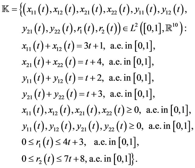
In the previous papers [1] and [2], a general equilibrium model of financial flows and prices is considered. The model is assumed evolving in time. The equilibrium conditions are considered in dynamic sense and the governing variational inequality formulation is presented. Precisely, the variational inequality we are working with is the following one:


where  is the set of feasible assets and liabilities for each sector
  given by

 is the total financial volume held by sector
  as assets,
  is the total financial volume held by sector
  as liabilities,
  is a measure of the risk of the financial agent,
  is the tax rate levied on sector
 ’s net yield on financial instrument
 is a nonnegative function,
  is the portion of financial transaction per unit employed to cover the expenses of the financial institutions,
  is the set of feasible instrument prices given by

where  and
and  are assumed to be in
 .
.
Setting, for the sake of simplicity,
defined as:
 (1)
(1)
 (2)
(2)
then variational inequality (1) becomes the problem:

Variational inequality (1) proved to be a very useful tool which enables us to study the financial equilibrium of an economy evolving in time and in the previous papers [1] and [2] the authors provided an interesting and useful output as the deficit formula, a general balance law and the liability formula which could be of great importance for the theory of equilibrium problems evolving in time. For the reader’s convenience we recall such important formulas:
1) Deficit formula
where  and
and  are the Lagrange variables associated to the price bounds:

The meaning of  is that it represents the deficit per unit whereas
  is the positive surplus per unit;
2) Balance law
3) Liability formula
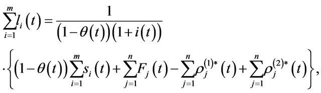
where  and
and  are the averages of
  and
and
 , namely
  and
and
 , respectively.
These suggested formulas could be of topical utility for the management of the world economy and to this aim in [2] the authors give some suggestions for the achievement of the world financial equilibrium and for finding the necessary way to follow in order to reach an improvement of the economy. It is worth reminding such suggestions:
Proposition 1.1 When the prices are minimal, namely they coincide with the floor prices, the economy collapses.
Proposition 1.2 Minimal prices imply the increase in the public debt.
Proposition 1.3 Minimal prices produce an economic recession. There is no incentive to the economic efforts.
Proposition 1.4 Even if it could be shocking, the development of the economy and of the employment results from an increase in the prices.
The value of these propositions can be realized by taking into account that the increase in prices indicated in Proposition 1.4 has been forecasted many months before (June 2011) it happened in our days.
Moreover, in [2] an “Evaluation Index”, that we denoted by , has been introduced as a useful and simple tool for the evaluation of an economy, given by
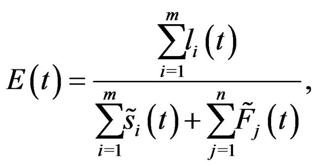
where we set

We remark that if  is greater or equal to 1 the evaluation of the financial equilibrium is positive (better if
  is proximal to 1) whereas if
  is less than 1 the evaluation of the financial equilibrium is negative.
The aim of this paper is to provide new theoretical and numerical results about solutions of financial equilibrium problems. In particular, we will prove a continuity result with respect to time of the solution, namely:
Theorem 1.1 Let , let
, let
 , let
, let  and let
 be a strongly monotone mapnamely there exists
  such that, for
 ,
,
Then variational inequality (1) admits a unique continuous solution.
Furthermore, we prove the following Lipschitz continuity result:
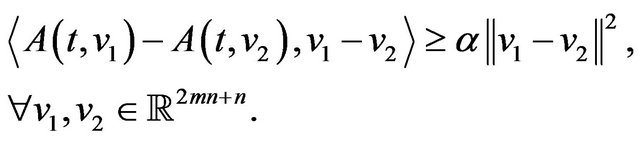
Theorem 1.2 Let  be strongly monotone, namely there exists
  such that, for
Lipschitz continuous with respect to , namely there exists
  such that, for

and Lipschitz continuous with respect to , namely there exists
  such that, for

Let  be two Lipschitz continuous functions and let
  be two Lipschitz continuous functions. Then, the unique financial equilibrium solution
  is Lipschitz continuous in
 . Moreover, let
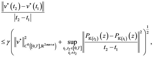
 , the following estimate holds:
 (3)
(3)
where  and
and

The continuity and Lipschitz continuity of solutions to financial equilibrium problems is a very important property for applications. Indeed, it is fundamental to establish numerical approximate solutions. Such numerical solutions can be obtained making use of a modified version of the algorithms (see for instances [3-7]). It is worth remarking that the Lipschitz continuity allows us to calculate the error in approximating the solution.
In order to clearly illustrate theoretical results, some significant examples are provided and, in such a way, the impact that the components of the model have on the equilibrium are highlighted.
It is worth mensioning that even in this case variational inequalities are able to express the time-dependent equilibrium conditions. Then, applying delicate tools of nonlinear analysis (see [8-11]), it is possible to prove existence results and qualitative analysis. For other economic problems where the time plays an important role we refer to the papers devoted to the Walrasian equilibrium problem [12-15], to the oligopolistic market equilibrium problem [16,17], to the weighted traffic equilibrium problem [18,19], and to [20].
The paper is organized as follows. In Section 2 we present the general financial model. In Section 3 we study the continuity results of the solution to the variational inequality which characterizes the financial model. In Section 4 we provide a Lipschitz continuity result for the solution. Finally, in Section 5 we propose a numerical examples from which we deduce that the solution, computed by means of the direct method (see [21]), is Lipschitz continuous.
2. The Model
We consider a financial economy consisting of  sectors, with a typical sector denoted by
 , and of
  instruments, with a typical financial instrument denoted by
 , in the time interval
 . Let
. Let  denote the total financial volume held by sector
  at time
  as assets, and let
  be the total financial volume held by sector
  at time
  as liabilities. Then, unlike previous papers (see [22-27]), we allow markets of assets and liabilities to have different investments
  and
and  respectively. Since we are working in the presence of uncertainty and of risk perspectives, the volumes
  and
and  held by each sector cannot be considered stable with respect to time and may decrease or increase depending on unfavorable or favorable economic conditions. At time
 , we denote the amount of instrument
  held as an asset in sector
 ’s portfolio by
  and the amount of instrument
  held as a liability in sector
 ’s portfolio by
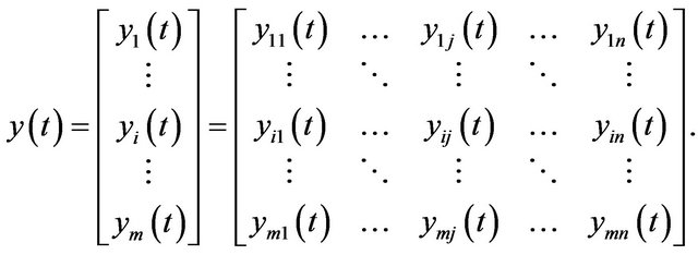
 . The assets and liabilities in all the sectors are grouped into the matrices

and
We denote the price of instrument j held as an asset at time t by  and the price of instrument j held as a liability at time
  by
by , where h is a nonnegative function defined into
  and belonging to
 . We introduce the term
  because the prices of liabilities are generally greater than or equal to the prices of assets so that we can describe, in a more realistic way, the behaviour of the markets for which the liabilities are more expensive than the assets. In such a way, this paper appears as an improvement in various directions of the previous ones [22-27]. We group the instrument prices held as assets into the vector
 and the instrument prices held as liabilities into the vector

In our problem the prices of each instrument appear as unknown variables. Under the assumption of perfect competition, each sector will behave as if it has no influence on the instrument prices or on the behaviour of the other sectors.
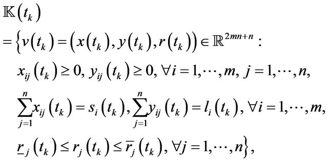
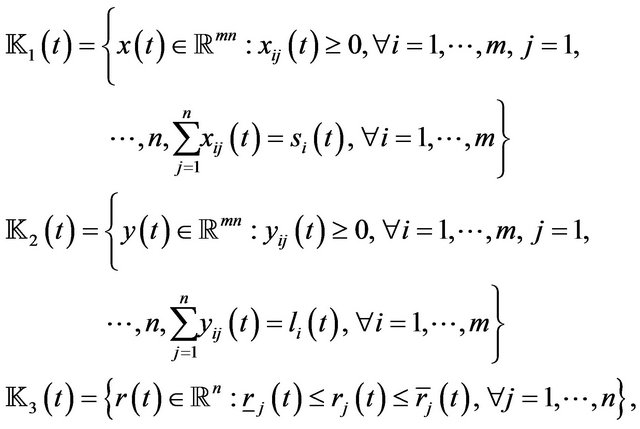
In order to express the time-dependent equilibrium conditions by means of an evolutionary variational inequality, we choose as a functional setting the very general Lebesgue space . Then, the set of feasible assets and liabilities for each sector
 , is
, is 
Now, in order to improve the model of competitive financial equilibrium described in [1], we consider the possibility of policy interventions in the financial equilibrium and incorporate them in form of taxes and price controls.
To this aim, denote the ceiling price associated with instrument  by
by  and the nonnegative floor price associated with instrument
  by
by , with
 , a.e. in
 . The meaning of the constraint
  a.e. in
  is that to each investor a minimal price
  for the assets held in the instrument
  is guaranteed, whereas each investor is requested to pay for the liabilities not less than the minimal price
 . Analogously each investor cannot obtain for an asset a price greater than
  and as a liability the price cannot exceed the maximum price
 .
.
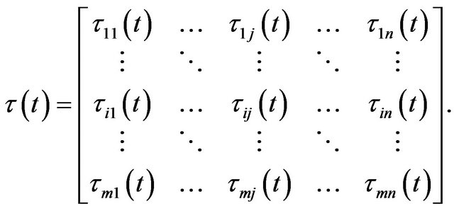
Denote the given tax rate levied on sector ’s net yield on financial instrument
 , as
, as . Assume that the tax rates lie in the interval
  and belong to
  . Therefore, the government in this model has the flexibility of levying a distinct tax rate across both sectors and instruments.
Let us group the instrument ceiling prices  into the column vector
 , the instrument floor prices
  into the column vector
 , and the tax rates
  into the matrix
The set of feasible instrument prices is 
In order to determine for each sector  the optimal composition of instruments held as assets and as liabilities, we consider, as usual, the influence due to riskaversion and the process of optimization of each sector in the financial economy, namely the desire to maximize the value of the asset holdings and to minimize the value of liabilities. Then, we introduce the utility function
 , for each sector
 , in this way
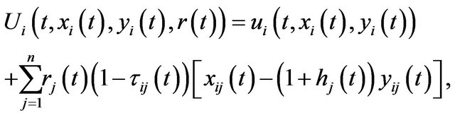
where the term  represents a measure of the risk of the financial agent and
 represents the value of the difference between the asset holdings and the value of liabilities. We suppose that the sector’s utility function
  is defined on
 , is measurable in
  and is continuous with respect to
  and
and . Moreover we assume that
  and
and  exist and that they are measurable in
  and continuous with respect to
  and
and . Further, we require that
 and a.e. in
  the following growth conditions hold true:
 (4)
(4)
and
 (5)
(5)
where ,
,  ,
,  are non-negative functions of
 . Finally, we suppose that the function
 is concave.
In order to determine the equilibrium prices, we establish the equilibrium condition which expresses the equilibration of the total assets, the total liabilities and the portion of financial transactions per unit  employed to cover the expenses of the financial institutions including possible dividends, as in [1]. Hence, the equilibrium condition for the price
  of instrument
  is the following:
 (6)
(6)
In other words, the prices are determined taking into account the amount of the supply, the demand of an instrument and the charges , namely if there is an actual supply excess of an instrument as assets and of the charges
  in the economy, then its price must be the floor price. If the price of an instrument is greater than
 , but not at the ceiling, then the market of that instrument must clear. Finally, if there is an actual demand excess of an instrument as liabilities and of the charges
  in the economy, then the price must be at the ceiling.
Now, we can give different but equivalent equilibrium conditions, each of which is useful to illustrate particular features of the equilibrium.
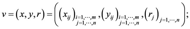
Definition 2.1 A vector of sector assets, liabilities and instrument prices  is an equilibrium of the dynamic financial model if and only if
 and a.e. in
  it satisfies the system of inequalities
 (7)
(7)
 (8)
(8)
and equalities
(9)
(10)
where  are Lagrange functions, and verify conditions (6) a.e. in
 .
.
Let us explain the meaning of the above conditions. To each financial volumes  and
and  held by sector
 , we associate the functions
 , related, respectively, to the assets and to the liabilities and which represent the “equilibrium disutilities” per unit of the sector
 . Then, (7) and (9) mean that the financial volume invested in instrument
  as assets
  is greater than or equal to zero if the
  -th component
 of the disutility is equal to
 , whereas if
 , then
 . The same occurs for the liabilities and the meaning of (6) is already illustrated.
The functions  and
and  are Lagrange functions associated a.e. in
  with the constraints
 and
and , respectively. They are unknown a priori, but this fact has no influence because we will prove in the following theorem that Definition is equivalent to a variational inequality in which
  and
and  do not appear.
Theorem 2.1 A vector  is a dynamic financial equilibrium if and only if it satisfies variational inequality (1).
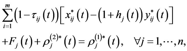
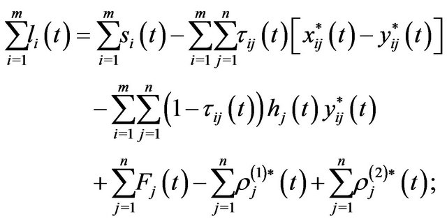
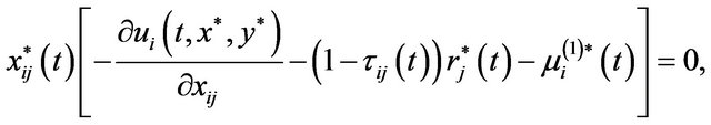
Moreover, we recall the result about Lagrange multipliers (see [2]):
Theorem 2.2 Let 
be a solution to variational inequality (1). Then there exist
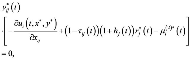
such that a.e. in ,
,
 (11)
(11)
 (12)
(12)
 (13)
(13)
 (14)
(14)
3. Continuity Results for Financial Equilibrium Solutions
In order to show the continuity result for the financial equilibrium problem, first of all, let us recall the wellknown property of set convergence due to K. Kuratowski (see [28]), that is a generalization of the classical Hausdorff definition of a metric for the space of closed subsets of a (compact) metric space.
Let  be a metric space and let
  be a sequence of subsets of
 . Recall that

where eventually means that there exists  such that
  for any
 , and frequently means that there exists an infinite subset
  such that
  for any
 . Finally we can remind the set convergence in Kuratowski’s sense.
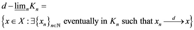
Definition 3.1 We say that  converges to some subset
  in Kuratwoski’s sense, and we briefly write
 , if
, if . Thus, in order to verify that
 , it suffices to check that
(K1) , i.e. for any
 , there exists a sequence
  converging to x in X such that
  lies in
  for all
 ;
;
(K2) , i.e. for any subsequence
 converging to x in X, such that
  lies in
for all , then the limit
  belongs to
 .
.
Now, let us prove that the set of feasible vectors satisfies the property of the set convergence in Kuratowski’s sense.
Proposition 3.1 Let , let
, let
 , let
, let  and let
 be a sequence such that
 , as
, as . Then, the sequence of sets
 , converges to

as , in Kuratowski’s sense.
Proof In order to prove that the sequence  converges to
  in Kuratowski’s sense, for any sequence
  such that
 , as
, as , it is enough to show that conditions (K1) and (K2) hold.
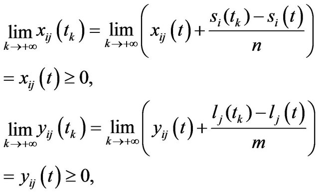
Let  be fixed and let us consider the sequence
 , such that
 ,
,  ,
,  ,
,

and ,
,  ,
,

Let us verify that ,
, . Taking into account that
there exist two index  and
and  such that for
  we get

and for  we have
Since ,
,
 , it results
 ,
, . Moreoverbeing
 ,
,
 , it follows
 ,
, . Finally, it results

Then we can consider a sequence  such that for
 ,
,  ,
,  ,
,
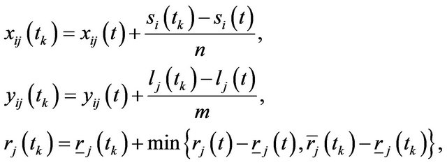
and for ,
,  ,
,  ,
,
where  denotes the Hilbertian projection on
 .
.
We have  and for
Then the first condition has been shown.
For the second one, let  be a fixed sequence, with
 ,
,
 , such that
  in
in ,
,
 in
in ,
,  in
in . We want to prove that
 . Since
 ,
,  , it results
 (15)
(15)
 (16)
(16)
 (17)
(17)
Passing to the limit as  in (15), (16) and (17), we obtain

Then .
.
The claim is, now, achieved.□
For what follows, it is convenient to recall that variational inequality (1) can be rewritten in the equivalent parameterized form:
 (18)
(18)
where the constraint set ,
,  , is a closed convex and nonempty subset of
 ,
,
 is a mapping and
  denotes the scalar product in
 . Moreover, we recall that under general assumptions existence theorems have been proved in [2] (see Section 6).
Taking into account the general continuity result for solutions to parameter variational inequalities in reflexive Banach spaces (see [29], Theorem 4.1) and Proposition, we obtain Theorem 1.1 of Section 1.
Theorem 1.1 Let , let
, let
 , let
, let  and let
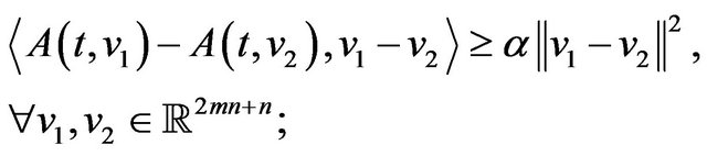
 be a strongly monotone map, namely there exists
  such that, for
 ,
,

Then variational inequality (1) admits a unique continuous solution.
4. Lipschitz Continuity Result
The aim of this section is to provide a Lipschitz continuity result for the financial equilibrium solution. For this reason, we recall a general result proved in [30] for the solutions to the parameterized variational inequality (18). More precisely, the following result holds (see [30], Theorem 1):
Theorem 4.1 Let  be strongly monotone, Lipschitz continuous with respect to
 , Lipschitz continuous with respect to
 , and there exists
  such that, for
 ,
,

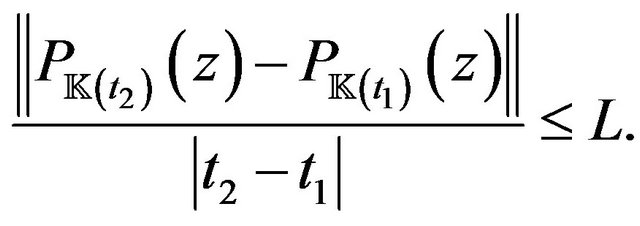
where ,
,  , denotes the projection onto the set
 . Then, the unique solution
 ,
,  , to (18) is Lipschitz continuous in
 ,
,  , the following estimate holds:
where .
.
For the sake of simplicity, we set
 .
.
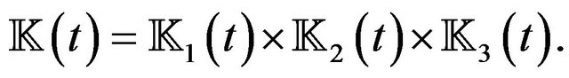
Before applying the previous result to our dynamic financial equilibrium problem, it is necessary to estimate the variation rate of projections onto time-dependent constraint set  describing the problem. It is useful to note that
  can be rewritten as the Cartesian product of the following set:
namely
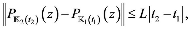
Making use of Proposition 1 in [30], we can show that assuming ,
,  , is Lipschitz continuous with Lipschitz constant
 , for
, for , it results
 (19)
(19)
Moreover, under the assumption that ,
,  , is Lipschitz continuous with Lipschitz constant
 , for
, for , we have
 (20)
(20)
Now, taking into account Proposition 4.1 in [31] and assuming that  and
and ,
,  , are Lipschitz continuous with Lipschitz constants
  and
and , respectively, for
 , we can prove
 (21)
(21)
where .
.
We can conclude that Proposition 4.1 Let , let
, let  be two Lipschitz continuous functions and let
  be two Lipschitz continuous functions. Let
  be an arbitrary point in
 . Then it results to be
where  is the positive constant as in (3).
As a consequence, it results
Hence, applying Theorem 4.1, we get the following result.
Theorem 1.2 Let  be strongly monotone (with constant
 ), Lipschitz continuous with respect to
  (with constant
 ), Lipschitz continuous with respect to
  (with constant
 ), and let
  be two Lipschitz continuous functions and let
  be two Lipschitz continuous functions. Then, the unique financial equilibrium solution
  is Lipschitz continuous in
 . Moreover, let
 , the following estimate holds:
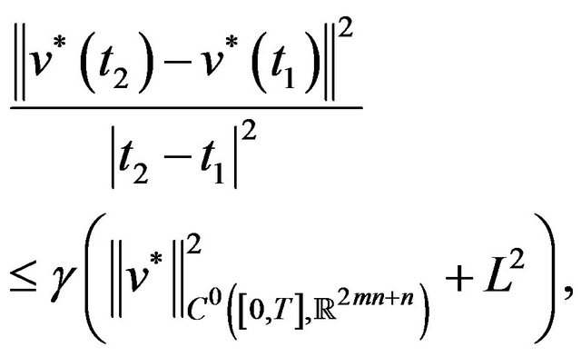
where .
.
5. Some Numerical Examples
Let us study some numerical financial examples in which we consider as the risk aversion function the one suggested by H.M. Markowitz in [32] and [33], which expresses at each instant  the risk aversion by means of variance-covariance matrices denoting the sector’s assessment of the standard deviation of prices for each instrument. We will see that the solutions of the examples are regular and we illustrate the impact of the components of the model on the financial equilibrium, especially for what regards
  and
and  and the deficit and the surplus.
Let us consider an economy with two sectors and two financial instruments, as shown in Figure 1, but this setting is not restrictive since we can consider a general economy by an iteration of this significant case, and assume that the variance-covariance matrices of the two sectors are the following:
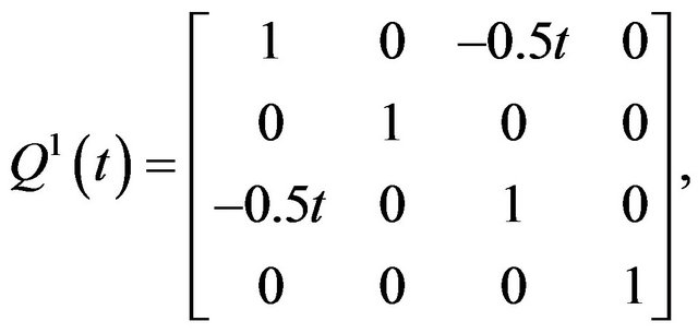
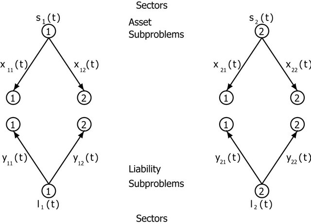
Figure 1. Two sectors and two financial instruments network a.e. in [0,1].

Let us choose as the feasible set
The variational inequality
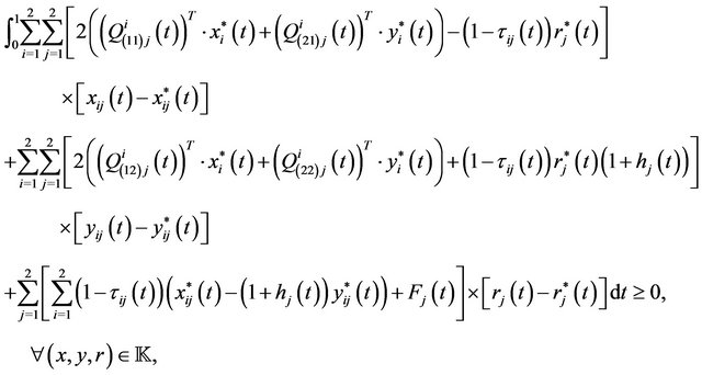
which expresses the financial equilibrium conditions, becomes
 (22)
(22)
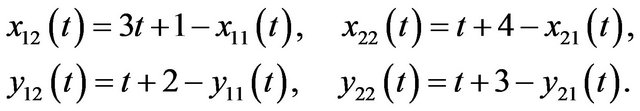
Following the direct method (see [21]) in order to find the solution, we can derive from the constraints of the convex set  the values of some variables in terms of the others, namely we obtain, a.e. in
 ,
,
Then, setting
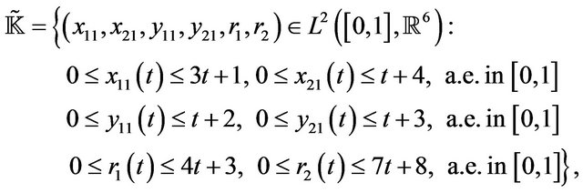
variational inequality (22) can be expressed in the equivalent form:

Let us set


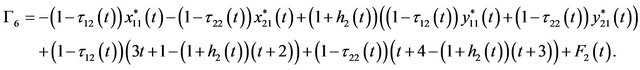
As the first step of the direct method suggests, let us search solutions obtained from the system

We get the values of the variables  and
and  in terms of
  and
and , namely
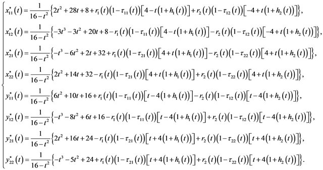
For the sake of simplicity, we assume
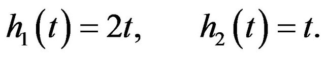
We get

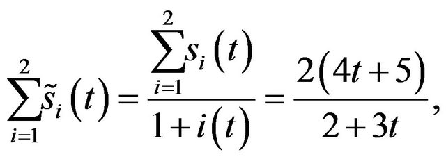
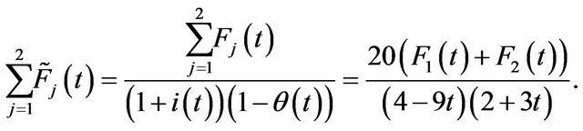
In the following, we study various examples of financial equilibrium for which the deficit (namely ) and surplus (namely
 ) are different from zero in certain time intervals. Such examples depend on the choose of suitable values of the data. In the first example, we consider values of
  such that
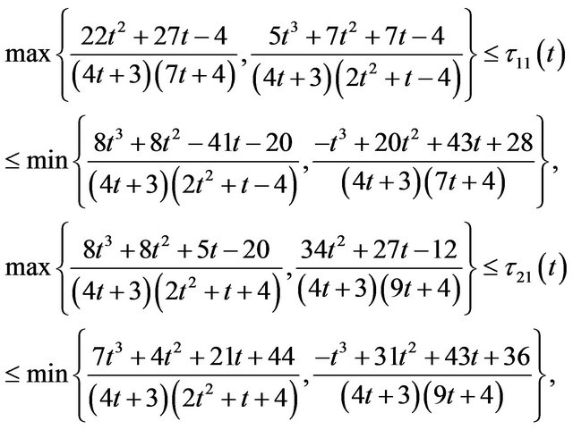
as Figures 2 and 3 show.
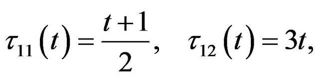
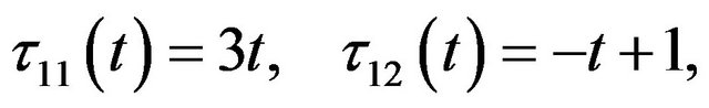
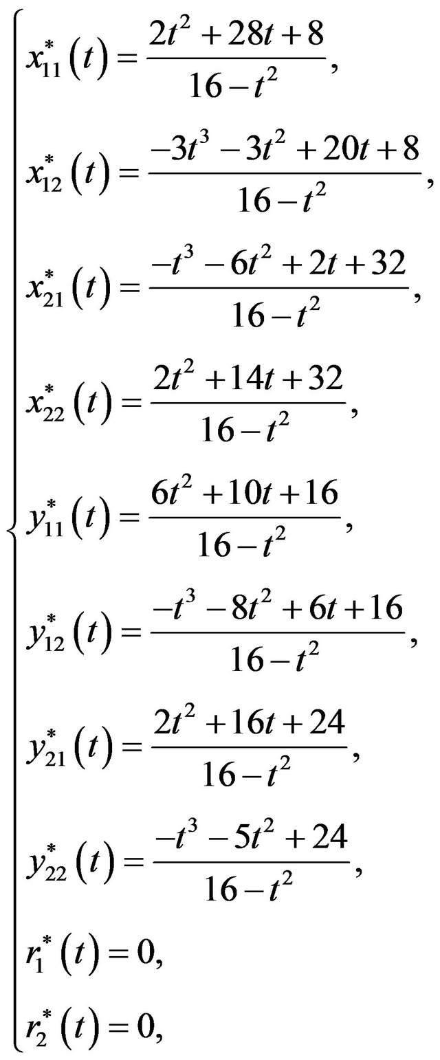
In particular, we assume

There exist  and
and , such that the vector
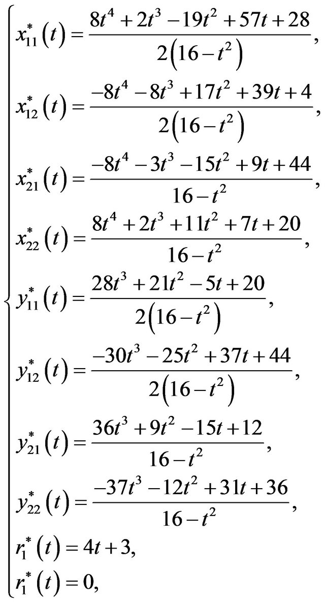
is solution of the variational inequality in the interval , because
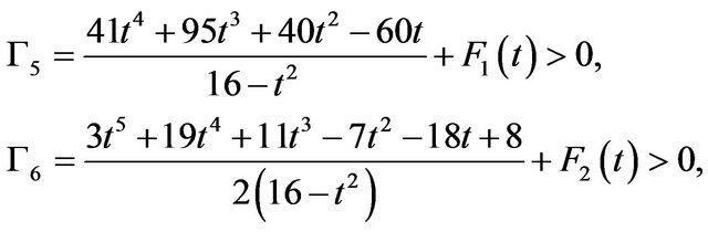
  fulfil the constraints and

Figure 2. Bound functions of .
.

Figure 3. Bound functions of .
.
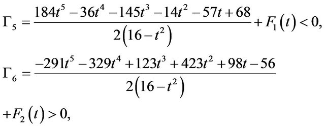
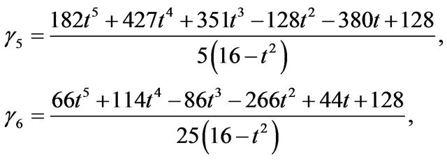
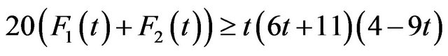
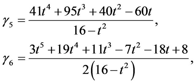
for  small enough and for any
  non negative. In fact, if we consider

we obtain that they are negative and positive respectively, as it can be verified in Figure 4 where the graphs of the numerators are represented.
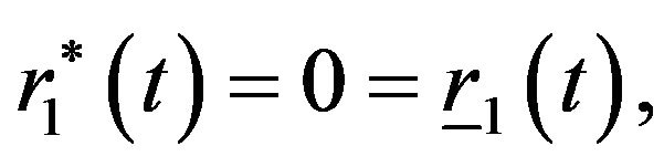
Let us remember that, by virtue of Theorem 2.2,  , the following relationships are satisfied
 (23)
(23)
 (24)
(24)
Taking into account that, in our case,

from (23), we obtain
So, from (24), we get
provided that  is small enough and for any
  non negative.
The importance of this example remains in the fact that, in the interval , for
, for  small enough, price
  is maximum and the financial market has a surplus given by


Figure 4.  and
and  in
in .
.
Whereas, for the instrument , we have minimal price and the deficit is given by
Now, we would like to calculate the Evaluation Index for this financial problem. More precisely, we have

As a consequence, the Evaluation Index is given by:

In the interval , if
, if

the economy has a positive average evaluation. The same situation happens if
in the interval  (where
 ).
).
Now let us consider the case where the values of  are such that

as Figures 5 and 6 show.
In particular, we assume

There exist  and
and , such that the vector

Figure 5.  and
and  in
in .
.

Figure 6.  and
and  in
in .
.
is solution of the variational inequality in the interval , because
  fulfil the constraints and
for any  non negative and for
  small enough. In fact, if we consider
we obtain that they are positive and negative respectively, as it can be verified in Figures 7 and 8 where the graphs of the numerators are represented in detail.
If we remember that, in this case,

from (23), we obtain


So, from (24), we get

provided that  is small enough and for any
  non negative.
In this situation, we can assert that, in the interval , for the instrument
 , we have minimal price and the deficit is given by

Whereas, for  small enough, price
  is maximum and the financial market has a surplus given by

Now let us proceed to the calculation of the Evaluation Index. We have

Then the Evaluation Index is


Figure 7.  and
and  in
in .
.

Figure 8.  and
and  in
in .
.
As a consequence, in the interval , if
, if

the economy has a positive average evaluation. The same situation happens if
in the interval  (where
 ). From this example we see that we can get useful information from the
 , which requires simple calculations.
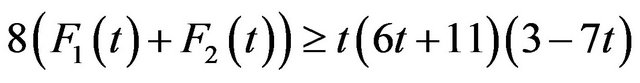
Now, we would like to study another example in which we assume

Under these assumptions, there exist  and
and , such that the vector
is solution of the variational inequality in the interval , because
  fulfil the constraints and
for  and
and  non negative. In fact, if we consider
we obtain that they are both positive, as it can be verified in Figure 9 where the graphs of the numerators are represented.
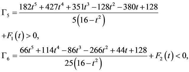
We observe that, in our case

so, from (23), it follows that

Then, from (24), we obtain


for any  and
and  non negative.
As consequence of the meaning of , in the interval
 , for both the instruments, we have minimal price and the deficit is given, respectively, by

As regards the calculation of the Evaluation Index, we have

Figure 9.  and
and  in
in .
.


As a consequence, the Evaluation Index is

Then, in the interval , if
, if
the economy has a positive average evaluation because . From this example we see that it is easier to achieve financial balance if
  and
and  are more or less equal.
REFERENCES
- A. Barbagallo, P. Daniele and A. Maugeri, “Variational Formulation for a General Dynamic Financial Equilibrium Problem. Balance Law and Liability Formula,” Nonlinear Analysis: Theory, Methods & Applications, Vol. 75, No. 3, 2012, pp. 1104-1123. doi:10.1016/j.na.2010.10.013
- A. Barbagallo, P. Daniele, S. Giuffrè and A. Maugeri, “Variational Approach for a General Financial Equilibrium Problem: the Deficit Formula, the Balance Law and the Liability Formula, a Path to the Economy Recover,” Submitted.
- A. Barbagallo, “Degenerate Time-Dependent Variational Inequalities with Applications to Traffic Equilibrium Problems,” Computational Methods in Applied Mathematics, Vol. 6, No. 2, 2006, pp. 117-133.
- A. Barbagallo, “Regularity Results for Time-Dependent Variational and Quasi-Variational Inequalities and Application to Calculation of Dynamic Traffic Network,” Mathematical Models and Methods in Applied Sciences, Vol. 17, No. 2, 2007, pp. 277-304. doi:10.1142/S0218202507001917
- A. Barbagallo, “Regularity Results for Evolutionary Nonlinear Variational and Quasi-Variational Inequalities with Applications to Dynamic Equilibrium Problems,” Journal of Global Optimization, Vol. 40, No. 1-3, 2008, pp. 29-39. doi:10.1007/s10898-007-9194-5
- A. Barbagallo, “Existence and Regularity of Solutions to Nonlinear Degenerate Evolutionary Variational Inequalities with Applications to Traffic Equilibrium Problem,” Applied Mathematics and Computation, Vol. 208, No. 1, 2009, pp. 1-13. doi:10.1016/j.amc.2008.10.030
- A. Barbagallo, “On the Regularity of Retarded Equilibria in Time-Dependent Traffic Equilibrium Problems,” Nonlinear Analysis, Vol. 71, No. 12, 2009, pp. e2406-e2417. doi:10.1016/j.na.2009.05.054
- P. Daniele and S. Giuffrè, “General Infinite Dimensional Duality and Applications to Evolutionary Network Equilibrium Problems,” Optimization Letters, Vol. 1, No. 3, 2007, pp. 227-243.
- P. Daniele, S. Giuffré and A. Maugeri, “Remarks on General Infinite Dimensional Duality with Cone and Equality Constraints,” Communications in Applied Analysis, Vol. 13, No. 4, 2009, pp. 567-578.
- P. Daniele, S. Giuffrè, G. Idone and A. Maugeri, “Infinite Dimensional Duality and Applications,” Mathematische Annalen, Vol. 339, No. 1, 2007, pp. 221-239. doi:10.1007/s00208-007-0118-y
- A. Maugeri and F. Raciti, “Remarks on Infinite Dimensional Duality,” Journal of Global Optimization, Vol. 46, No. 4, 2010, pp. 581-588. doi:10.1007/s10898-009-9442-y
- M. B. Donato, M. Milasi and C. Vitanza, “Dynamic Walriasian Price Equilibrium Problem: Evolutionary Variational Approach with Sensitivity Analysis,” Optimization Letters, Vol. 2, No. 1, 2008, pp. 113-126. doi:10.1007/s11590-007-0047-4
- M. B. Donato, M. Milasi and C. Vitanza, “Quasi-Variational Approach of a Competitive Economic Equilibrium Problem with Utility Function: Existence of Equilibrium,” Mathematical Models and Methods in Applied Sciences, Vol. 18, No. 3, 2008, pp. 351-367. doi:10.1142/S0218202508002711
- M. B. Donato, A. Maugeri, M. Milasi and C. Vitanza, “Duality Theory for a Dynamic Walrasian Pure Exchange Economy,” Pacific Journal of Optimization, Vol. 4, No. 3, 2008, pp. 537-547.
- M. B. Donato, M. Milasi and C. Vitanza, “A New Contribution to a Dynamic Competitive Equilibrium Problem,” Applied Mathematics Letters, Vol. 23, No. 2, 2010, pp. 148-151. doi:10.1016/j.aml.2009.09.002
- A. Barbagallo and M.-G. Cojocaru, “Dynamic Equilibrium Formulation of Oligopolistic Market Problem,” Mathematical and Computer Modelling, Vol. 49, No. 5-6, 2009, pp. 966-976. doi:10.1016/j.mcm.2008.02.003
- A. Barbagallo and A. Maugeri, “Duality Theory for the Dynamic Oligopolistic Market Equilibrium Problem,” Optimization, Vol. 60, No. 1-2, 2011, pp. 29-52. doi:10.1080/02331930903578684
- S. Giuffrè and S. Pia, “Weighted Traffic Equilibrium Problem in Non Pivot Hilbert Spaces,” Nonlinear Analysis, Vol. 71, No. 12, 2009, pp. e2054-e2061. doi:10.1016/j.na.2009.03.044
- A. Barbagallo and S. Pia, “Weighted Variational Inequalities in Non-Pivot Hilbert Spaces with Applications,” Computational Optimization and Applications, Vol. 48, No. 3, 2011, pp. 487-514. doi:10.1007/s10589-009-9259-0
- S. Giuffrè, G. Idone and S. Pia, “Some Classes of Projected Dynamical Systems in Banach Spaces and Variational Inequalities,” Journal of Global Optimization, Vol. 40, No. 1-3, 2008, pp. 119-128. doi:10.1007/s10898-007-9173-x
- A. Maugeri, “Convex Programming, Variational Inequalities and Applications to the Traffic Equilibrium Problem,” Applied Mathematics & Optimization, Vol. 16, No. 2, 1987, pp. 169-185. doi:10.1007/BF01442190
- P. Daniele, “Variational Inequalities for Evolutionary Financial Equilibrium,” In: A. Nagurney, Ed., Innovations in Financial and Economic Networks, Edward Elgar Publishing, Cheltenham, 2003, pp. 84-108.
- P. Daniele, “Variational Inequalities for General Evolutionary Financial Equilibrium,” In: F. Giannessi and A. Maugeri, Eds., Variational Analysis and Applications, Springer Verlag, New York, 2005, pp. 279-299.
- P. Daniele, “Evolutionary Variational Inequalities Applied to Financial Equilibrium Problems in an Environment of Risk and Uncertainty,” Nonlinear Analysis, Vol. 63, No. 5-7, 2005, pp. 1645-1653.
- P. Daniele, “Dynamic Networks and Evolutionary Variational Inequalities,” Edward Elgar Publishing, Chentelham, 2006.
- P. Daniele, “Evolutionary Variational Inequalities and Applications to Complex Dynamic Multi-Level Models,” Transportation Research Part E, Vol. 46, No. 6, 2010, pp. 855-880. doi:10.1016/j.tre.2010.03.005
- P. Daniele, S. Giuffrè and S. Pia, “Competitive Financial Equilibrium Problems with Policy Interventions,” Journal of Industrial and Management Optimization, Vol. 1, No. 1, 2005, pp. 39-52. doi:10.3934/jimo.2005.1.39
- K. Kuratowski, “Topology,” Academic Press, New York, 1966.
- A. Barbagallo and M.-G. Cojocaru, “Continuity of Solutions for Parametric Variational Inequalities in Banach Space,” Journal of Mathematical Analysis and Applications, Vol. 351, No. 2, 2009, pp. 707-720. doi:10.1016/j.jmaa.2008.10.052
- A. Maugeri and L. Scrimali, “Global Lipschitz Continuity of Solutions to Parameterized Variational Inequalities,” Bollettino Unione Matematica Italiana, Vol. 2, No. 9, 2009, pp. 45-69.
- A. Barbagallo and R. Di Vincenzo, “Lipschitz Continuity and Duality for Dynamic Oligopolistic Market Equilibrium Problem with Memory Term,” Journal of Mathematical Analysis and Applications, Vol. 382, No. 1, 2011, pp. 231-247. doi:10.1016/j.jmaa.2011.04.042
- H. M. Markowitz, “Portfolio Selection,” The Journal of Finance, Vol. 7, No. 1, 1952, pp. 77-91.
- H. M. Markowitz, “Portfolio Selection: Efficient Diversification of Investments,” Wiley, New York, 1959.