Abstract

This paper provides a detailed outline of a mathematical research exploration for use in an introductory high school or college Calculus class and is directed toward teachers of such courses. The discovery is accomplished by introducing a novel method to generate a polynomial expression for each of the Euler sums,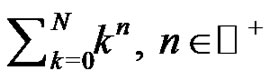. The described method flows simply from initial discussions of the Riemann sum definition of a definite integral and is readily accessible to all new calculus students. Students investigate the Bernoulli numbers and the interesting connections with Pascal's Triangle. Advice is offered throughout as to how the project can be assigned to students and offers multiple suggestions for additional exploration for any motivated student.

1. Introduction

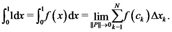
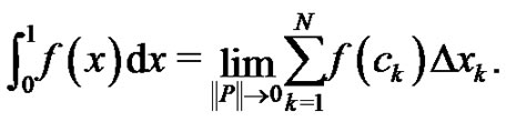
During the initial discussion of a Riemann sum in a two year high school or one year college Calculus sequence, the Riemann definition of a definite integral,

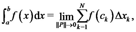(1)

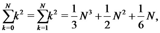
where is a partition of the closed interval, is the length of the subinterval , and is the norm of the partition (the largest subinterval width), is one of our first lessons once we begin the topic of integral calculus [1]. This definition naturally leads to a broad discussion of several common summations, including

We shall refer to these as the first three Euler sums. This connection between the Riemann sum and the Euler sums provides an opportunity to explore some interesting mathematics that students probably have not been exposed to, but is highly accessible and relevant to them from this direction. The exploration connects the topics of limits, integral calculus, linear algebra, the binomial coefficient, and number theory in a cohesive manner. The project gives the students motivation to learn the mathematics of these various areas. The purpose of the exercise described in this paper is to provide a chance for high school or college students to discover and validate for themselves the view that mathematics is a beautiful thing and is an incredibly rewarding achievement of mankind that is continuing to be created.

 An overarching theme for the entire paper is this work can be used by calculus teachers to provide a highly motivating example to explore the various fields of introductory mathematics by presenting a single problem illustrating the many connections among several branches of mathematics. A common experience will be to start the project with students who have no concept whatsoever as to what mathematical research even means, nor how to begin, and end the project with students who will not know how to stop their discovery. Along the way, the beauty in mathematics cannot help but shine bright. Examples, proofs, and explanations provided in this paper are presented in great detail to assist the fellow high school or college teacher in implementing the project.

This paper is organized as follows: In Section 2 a novel method to generate a polynomial expression for all of the Euler sums, 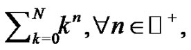from the Riemann definition of a definite integral is developed. In Section 3 the historical method developed by Jakob Bernoulli 300 years ago to generate the same polynomial expressions for these sums is outlined [2]. In Section 4 a connection is developed between the Riemann sum method and Bernoulli’s. The two methods are quite distinct, yet connections exist that will be explored. In Section 5 the developed Riemann sum method is shown to independently produce each of the Bernoulli numbers and each Euler sum with a simple recursive formula. Section 6 concludes the paper with a few final remarks.

2. The Riemann Method

By requiring students to work through finding

for simple functions such as or using the Riemann definition of the definite integral from (1), an interesting connection between the definite integral and the Euler sums develops, illustrated by the following series of examples:

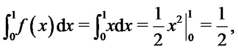
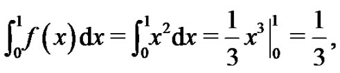
First, let It is known [3] that

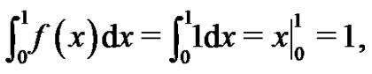
but, from (1) we also know

Partition the interval into equal width subintervals by choosing to be the left-hand point of each subinterval, Hence,where Notice that as Notice also that Therefore,

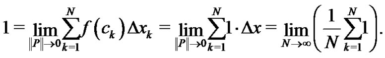
The last limit, namely, , is an indeterminate form. However, since we know its value is 1, the form of the summation inside the limit is determined. Clearly, must be of the form where is a constant yet to be calculated. By choosing a specific value of (e.g.,), the constant can easily be evaluated to find. So,

(2)

which will be no surprise to any of the students.

Next, let It is known [3] that

but, from (1) we know

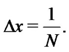Again, partition the interval into equal width subintervals by choosing to be the left-hand point of each subinterval Hence, once againwhere Notice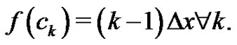Therefore,

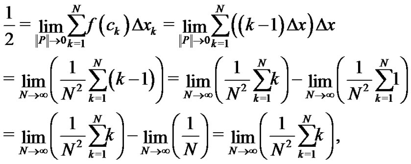
where we have used equation (2) and have evaluated the second limit. Using similar logic as in the previous example, 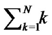must be of the form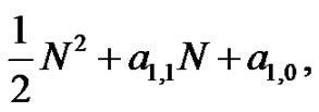where and are constants to be determined. By choosing specific values of (e.g.,) the constants and can easily be evaluated with a small system of equations

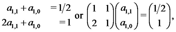
to find and The students are asked to evaluate this system of equations by hand. So,

(3)

a well known formula that the students will more than likely have previously seen [4], but found in a rather unique and back door manner that students find intriguing.

This analysis can be repeated by letting to determine as follows:

but, from (1) we know

Again, partition the interval as before into equal width subintervals by choosing to be the lefthand point of each subinterval Notice Therefore,

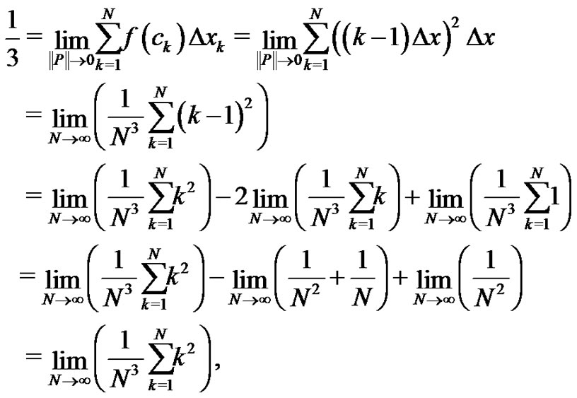
where we have used (2) and (3) in the last line above to simplify the limits. Therefore, must be of the form, where andare all constants to be determined. However, by choosing specific values of (e.g.,) the constants and can easily be evaluated with another small system of equations

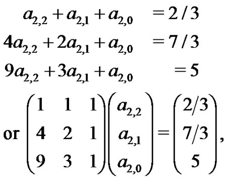
to fi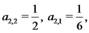nd and The students are asked to evaluate this system of equations by hand as well. By doing so, many students begin to see the patterns that develop even within these systems. They find

a relationship that simplifies to another well known formula, 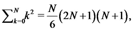that the students may also find familiar [4], but again found in a unique fashion. By now the students are generally quite curious about what lies ahead. In general

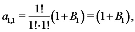
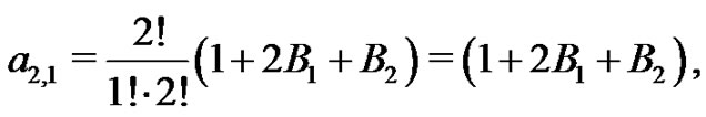
where is easily seen to be as a consequence of 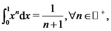and the remaining coefficients are found through simple linear algebra methods [5] as follows:

(4)

and hence,

where

and

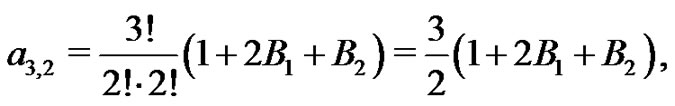
The recursive expressions above define the row and the column of the three matrices, and To serve as another example, with students will quickly find

Now, by evaluating this expression with and 5, (4) is used to determine the coefficients of from

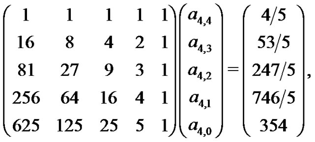
so that

or, and

. Without question, this method becomes cumbersome for large values of 1 Students quickly realize when solving the larger systems that the last column of in the above system is not necessary as the coefficient is easily shown to always be zero and does need to be calculated. This is trivial for, as for. Once this is realized, the system size drops by one and greatly simplifies the larger systems. However, we have found that it is best to let the students discover this on their own.

In this manner, all Euler sums can be generated for However, once grows to be in the ballpark of 10 or greater, the resulting matrices become badly scaled and ill-conditioned [6]. This idea is well beyond a student new to calculus, but by solving the systems of equations using these matrices one-by-one on a computer for larger and larger values of the students learn for themselves that the computer’s results begin to become inaccurate and are suspect. This is especially true when using software packages such as Matlab where the coefficients are all treated as real numbers. This discovery process is highly educational for the students as this may be their first situation in which the limits of a computer are very clear. Euler sums with very large values of will require a recursive relation which we develop in Section 5.

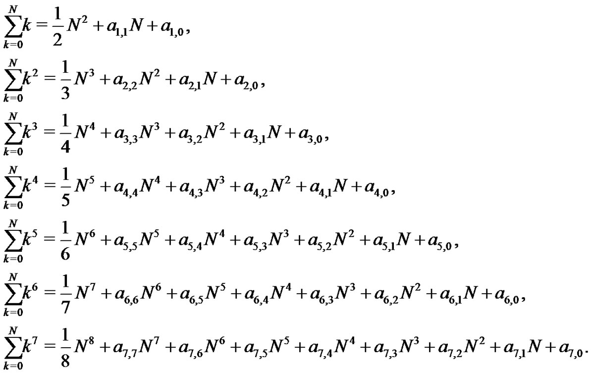
The students are next asked to generate the first ten Euler sums with this technique. splitting up the responsibilities or using a computer as time requirements demand. They are also asked to show,

and Then, by carefully organizing their results the students are challenged to extract patterns and investigate them to develop ideas on what is going on. They are encouraged to understand the structure and develop a way to predict higher order sums without the need to solve the larger and larger systems of equations. The students are given a hint by asking them to organize and present their results aligned in columns as shown below (See (5)).

From this form of presentation, the students will recognize many patterns right away. The first term is always the second term is always every other column is zero, the nonzero columns after the second column alternate in sign, the expressions all end with the term for even, and end with the term for odd. These patterns generate interest and motivation to understand what is generating them. It is fun for the students to experience this directly, and for the teacher to watch the students discover these many patterns.

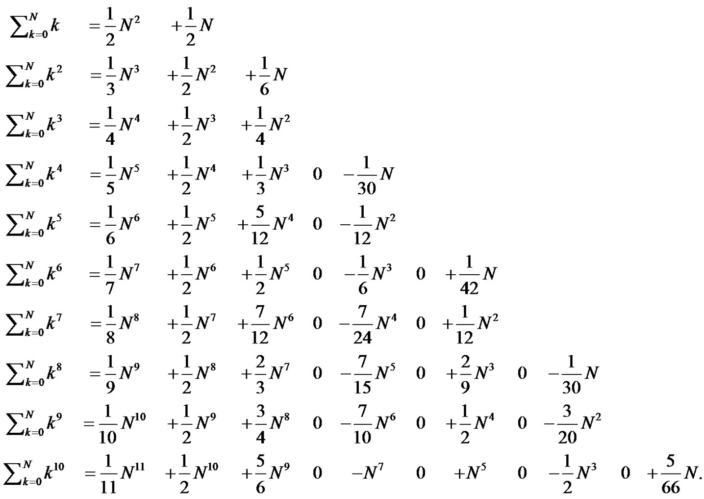(5)

Many open questions remain for the students to ponder at this point. Why are the zero columns being produced? Why is the sign alternating between the nonzero columns? These open questions provide ample opportunity for any motivated student to take this analysis as deeply as they desire. The students are challenged to find a general form for that may not require the solution of an system of equations.²

This project provides the students a universal view of mathematics - seeing how linear algebra comes into play, how calculus and simple number theory are connected. They quickly begin to see patterns forming which leads to various hypotheses about the structure of the connections. The intricate beauty that we all know is inherent in mathematics is demonstrated to the student with this exercise. Depending on one’s time constraints, the project could be ended at this point. However, a great many connections with history and other mathematical topics lie right around the corner.

3. The Bernoulli Method

This exercise provides a way to introduce another topic rarely visited by high school or new college students –  the Bernoulli polynomials and the Bernoulli numbers. It is fun for the students to step away from the text book for a breather now and then to gain a more global view of mathematics. We have found that providing connections between the various fields of mathematics gives students a more unified view of mathematics versus the common conception that most of what they learn over the years is a long series of unconnected material.

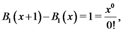
Our investigation into the Bernoulli numbers begins by explaining what the Bernoulli polynomials are and by giving one way in which they are commonly defined [7]. Let The students are asked to find the polynomial, satisfying the following conditions: 1), and 2). They quickly discover. 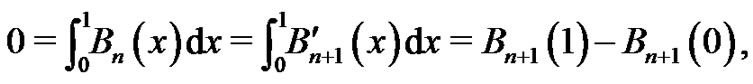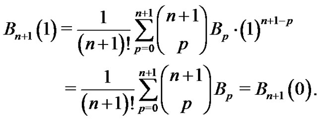The students are then asked to find the polynomial, satisfying the conditions: 1) and 2) They are asked to continue this process to generate these special polynomials up through All of these polynomials have the general properties that 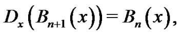and The first few of these polynomials are listed below (See (6)).

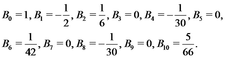
The polynomials the students generate are today known as one form of the Bernoulli polynomials, in honor of their discoverer, Jakob Bernoulli around the year 1700 [2]. In addition to the interesting properties discussed above which are used to generate them, they have an incredibly far reaching influence into the calculus and number theory. To begin to investigate a small part of their role, the students initially list the constant terms of the first few Bernoulli polynomials, through by evaluating each polynomial at. These constant terms are then used to calculate a new set of numbers, using the relationship

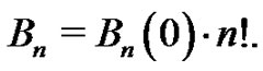(7)

In this manner, the students find what are known as the first few Bernoulli numbers:

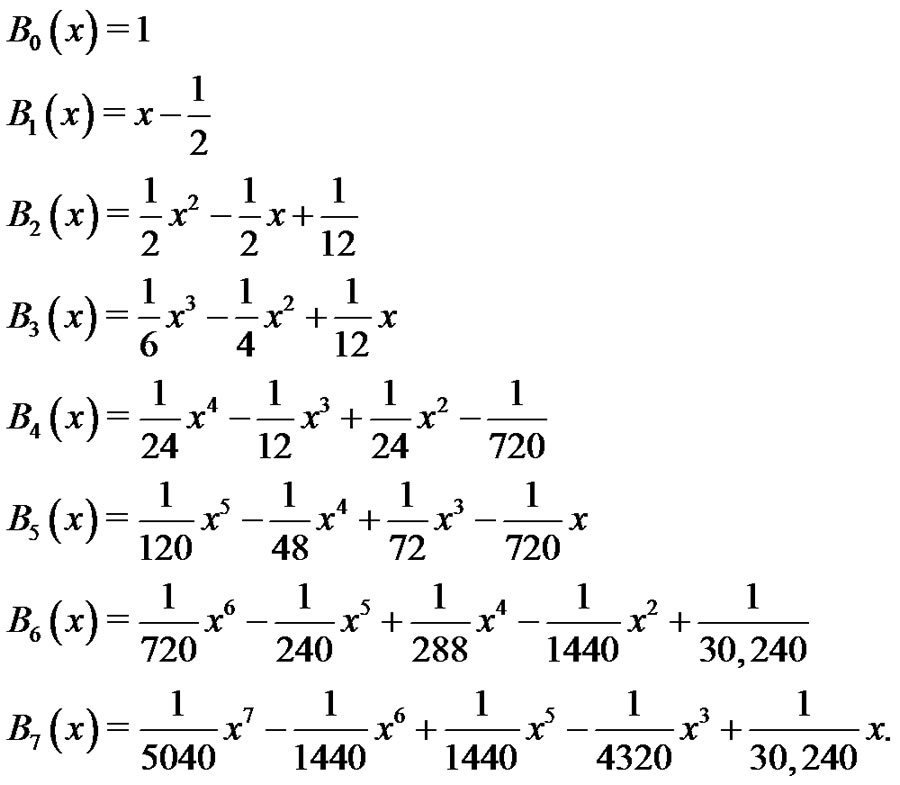(6)

Notice that refers to the Bernoulli polynomial and refers to the Bernoulli number, different quantities, but related through (7). The students generally notice that our original Riemann sum method is able to produce these Bernoulli numbers independently. One of the many interesting occurrences of the earlier method is that the coefficients of the Riemann method are each one of the Bernoulli numbers. In other words, ³ This sparks great interest in the students and they get a huge kick out of this.

The Bernoulli polynomials are especially easy to use when written in terms of the Bernoulli numbers. The first few polynomials are written below in this manner:

(8)

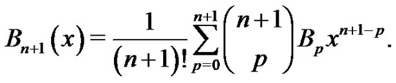
The standard compact form of the Bernoulli polynomials when written in this form is

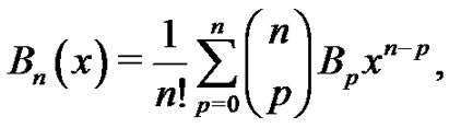(9)

where 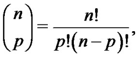is the standard binomial coefficient, but students generally need to be reminded of this notation.

Next, a connection between the Bernoulli Polynomials and the Euler Sums will be investigated. To begin, the students are gently guided through Bernoulli's important proof of a useful theorem.

Theorem: Let or zero, and let denote the Bernoulli Polynomial, then

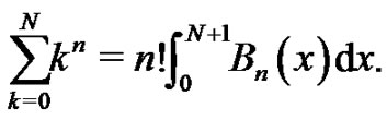(10)

Proof. We recall

by definition and by the Fundamental Theorem of Calculus. Therefore,

(11)

for any Writing (9) with instead of produces

Combining this result with (11) and evaluating at yields

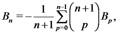
However, using (7) leads to

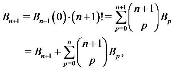
which is easily shown by expanding the summation. Hence,

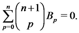(12)

This is a recursive relationship that allows one to generate the Bernoulli numbers starting with

Next, an important lemma will be proven that will be used to connect the Bernoulli polynomials with the Euler sums. The proof allows the students an opportunity to practice their induction techniques.

Lemma:

Proof. We will prove this lemma with a simple application of induction. Let From (8),

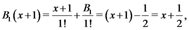
and

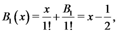
which agrees with (6). Therefore,

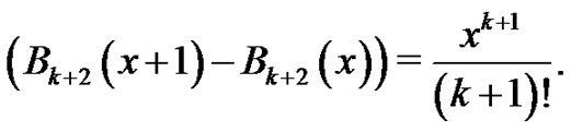
which verifies our base case. Now, assume as our induction hypothesis that

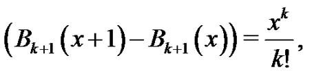
for some integer such that We need to show

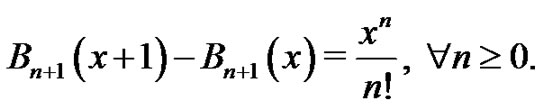
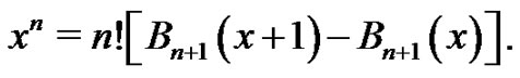
Recall the manner in which the Bernoulli polynomials are defined, namely,

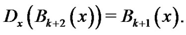
Therefore,

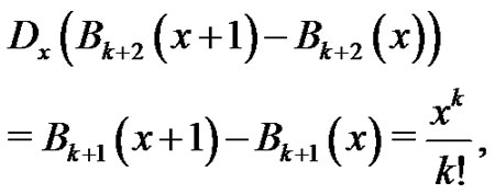
by hypothesis. So,

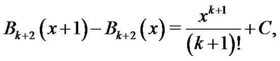
where is a constant of integration. However, when we have

from (11). Therefore, And so,

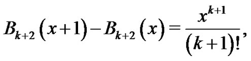
which is what we were trying to show. Hence, by the Principle of Mathematical Induction,

This completes the proof of the lemma.

The result of this lemma can alternatively be written as

(13)

Recall, and so, by the Fundamental Theorem of Calculus,

(14)

Finally, using (13) with and some fixed, one generates

which telescopes to produce

Now, using (14) we find our result:

which completes the proof of the main theorem.

The instructor may make as much of the previous section as they desire, perhaps making it a one day class driven proof after a detailed homework assignment from the previous evening. It certainly is a manageable proof, but just as certainly is not trivial. It has been our experience that initially the proof appears somewhat daunting, but once complete, the students are quite proud of their accomplishment and have gained considerable confidence in their abilities.

We then use the result of the theorem, (10), to generate the Euler sums in terms of the Bernoulli numbers. As an example, consider

Combining like terms yields

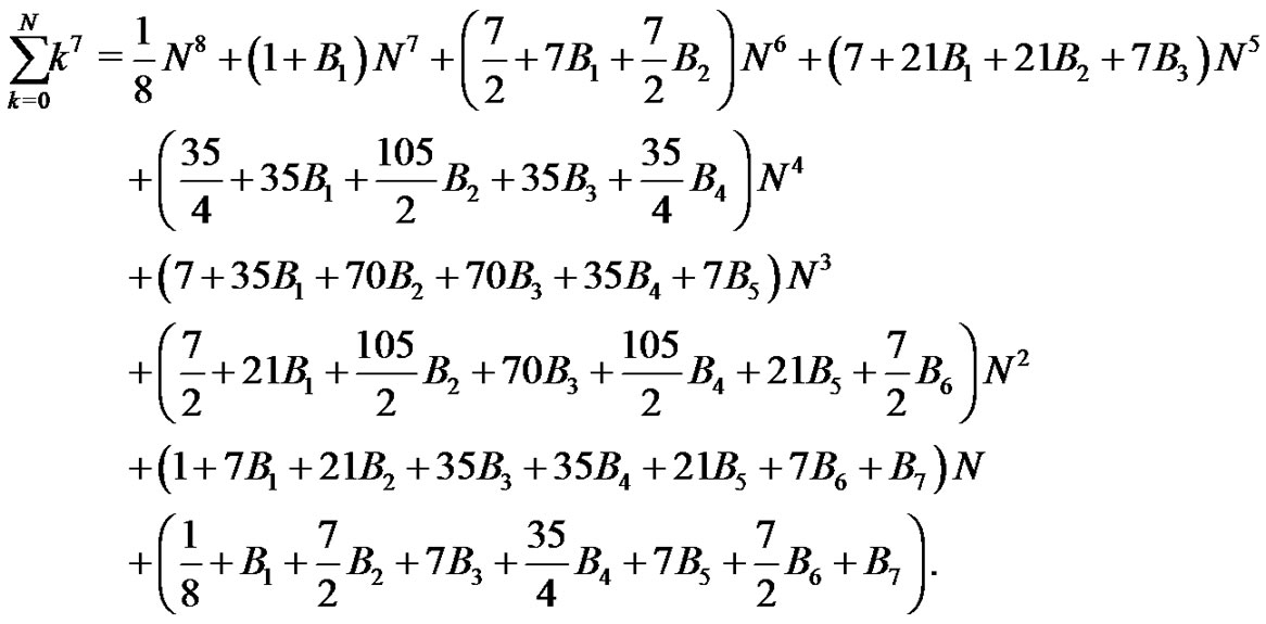(15)

We work through these integrals by hand, splitting up the work as necessary, and employing software such as Maple to help simplify the resulting expressions. The students get a nice practice session with simple integrals and are challenged with elementary algebra by trying to keep all of their terms consistent and organized. This process also reminds them that all of this work is intimately related to and connected with the calculus.

At this point in the project, the students have generated the first ten Euler sums with both the Riemann sum and the Bernoulli methods. The two sets of expressions are similar in that they are both sets of polynomials, however, they look quite distinct from one another. As an example, compare (5) for with (15).

Next, we investigate some of their many connections.

4. A Connection between the Riemann Sum Method and the Bernoulli Method

Comparing our initial Riemann sum form for the

sums from (5) to these new Bernoulli forms, as in (15), creates a set of incredible relationships that ignites the imagination. Notice that by comparing the new expressions, as in (15), to those generated using the Riemann sum idea, as in (5), a relationship between the coefficients and the Bernoulli numbers is determined. To illustrate, we write the first few Riemann sum method results in a more general form in terms of the coefficients:

(16)

Comparing all of the results for generated as was done in the previous section (i.e., (15)), with the corresponding expressions from the new Riemann method in (16), leads to a series of relationships between the coefficients and the Bernoulli numbers by equating coefficients term-by-term. As an example, for

(17)

Notice how (17) can be rewritten as

(18)

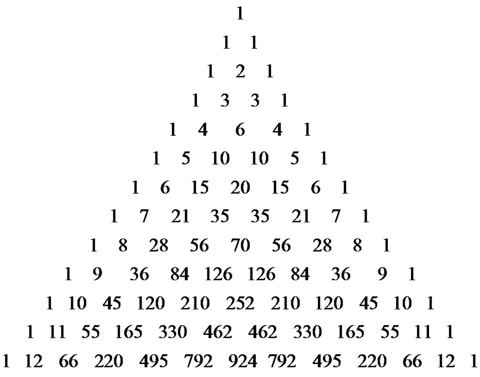
from which most students clearly see the Pascal Triangle coefficients emerging from the coefficients in the first seven lines of (18). This connection allows us to fully discuss the Pascal Triangle connections, the beautiful interplay that exists. As an example, compare the coefficients in (18) with the row of Pascal’s Triangle [8]:

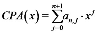
Clearly, the general form for the polynomial representation of the Euler sums derived through the previously described Riemann method is:

(19)

where the coefficients are related to the Bernoulli numbers by:

(20)

for with

(21)

for and respectively. All of which the students are asked to verify. Astute students will recognize that the first relation in (21) is (12). By introducing the binomial coefficient in this manner, students get a clear understanding of the meaning of the odd notation that is used to represent the factor. The patterns that are evident in (19) through (21) allows one to predict future coefficients in terms of higher order Bernoulli numbers as will be demonstrated in the next section.

This is another natural stopping point for the project. However, we have found many students feel compelled to follow the unfolding ideas more deeply. As an example, some may want to investigate on their own whether the polynomials we develop:

(22)

have special properties as do the Bernoulli polynomials. Students will investigate whether the Riemann sum idea can be used to generate the Euler sums for negative values of such as 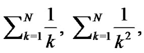and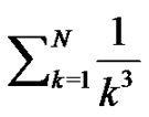

formulas as well. They ponder why the number does not seem to fit the general form for the generation of the Bernoulli numbers from the Riemann sum concept. Students develop explanations as to why the coefficient requires a separate definition from for They investigate the origin of the patterns generated throughout their work, such as why the coefficients in front of the Bernoulli equations agree with the coefficients in the equations term-by-term. Why do the zero columns in (5) exist? What causes the sign to alternate between nonzero columns? It has been our experience that students genuinely want to move in multiple directions at once and have a difficult time moving away from the investigation with questions left unanswered. We have succeeded in sparking their interest in mathematical research.

5. Independent Generation of the Bernoulli Numbers and Euler Sums

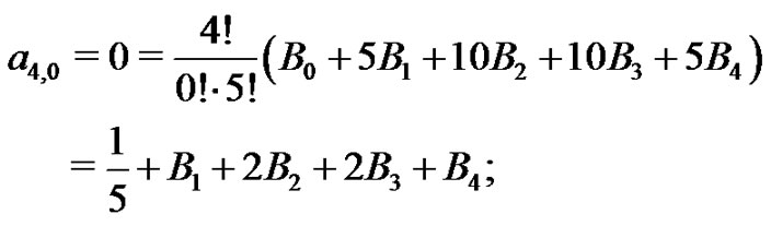
The students have already been encouraged to convince themselves, and prove that the term is always zero.⁴ By knowing they are able to generate all of the Bernoulli numbers from the Riemann sum method, a method very different from the initial construction of the Bernoulli numbers given by (12). They also see the recursive manner in which the Euler sums can be generated. To illustrate, several examples are detailed.

First, since the first Bernoulli number, is generated by taking the coefficient from the equivalent set of (18) expressions for Using (21) with they find:

Recalling from (20) that

or and so,

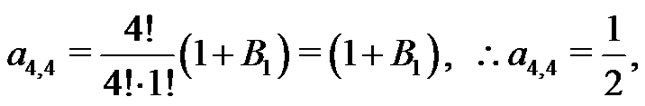
The students next see that using (21) with the second Bernoulli number, can be determined in a similar manner:

Again, recalling from (20) that

the students find

Also from (20),

and so,

Hence,

The third Bernoulli number, is found next. From (21) with

From (20), 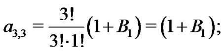hence,

Also,

and so,

Lastly,

yielding Therefore,

Now, so that the recursive method used to generate the Bernoulli numbers and the Euler sums from this new approach is clear, the case will also be shown in detail below and can be used as a template for even higher order Euler sums and Bernoulli numbers. From (21), with

therefore, 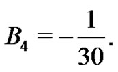The next step is to determine the

Euler sum by generating the coefficients one-by-one. Recall from (20) the following several results:

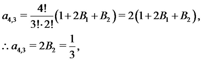
Hence,

This method is continued one at a time to find the next several Bernoulli numbers and Euler sums and can be used to generate them all. Following this idea, in general the required Bernoulli numbers are found from

(23)

which are then used with (19) through (21) to generate Euler sums for any Some students will notice that this technique to determine the Bernoulli numbers is essentially (12), but developed in a novel and independent manner that is readily accessible to new calculus students and intimately related to the integral.

Given our general form from (19) through (21), we can predict the values of higher order Bernoulli numbers through this recursive relationship without using (12). In fact, given this general recursive relationship, the students soon realize that each of the Euler sums, along with their respective set of coefficients, can be generated without the need to solve the earlier described system of equations which were becoming troublesome due to their large dimensions.

The students are asked to look up the known values of the Bernoulli numbers to validate their own independent generation of them. They are also asked to double check their generated formulas for the more complex Euler sums by hand with a few sample values for. As an example, with they will find, using the Riemann sum method, and the Euler sum to be:

It is a rewarding moment for all when the students validate their hard won expressions. This process solidly instills the importance of the unique set of Bernoulli number values and the interplay that exists. We doubt that any student who works through this exercise carefully will ever forget the Bernoulli number idea.

6. Concluding Remarks

The generation of the Euler sums from the Riemann definition of a definite integral provides an excellent vehicle to demonstrate the interplay of limits, integral calculus, number theory, linear algebra, binomial coefficients, recursive relationships, and Pascal’s Triangle. The project allows for discovery and a study of some interesting historical characters. It provides students a chance to experiment with mathematical research and allows them an opportunity to understand the importance of notation, how solving systems of equations is relevant, and how the Masters came onto these discoveries for themselves. It gives new students an opportunity to just “do some mathematics” and explore.

We feel the experience may give the students a taste of what or even century mathematics might have been like to actually live. They develop a sense of how a great deal of mathematical progress was made and many discoveries were uncovered by first looking for relationships and then digging in to explain and understand them.

This exercise would serve as an excellent ongoing “Math Club” type problem in which a motivated group of students may work on a bit of the problem each week and gradually discover many of the features of this problem on their own. This reasonably short excursion from a standard high school or introductory college calculus class will introduce the student to a wide array of new ideas and should aid in reinforcing the relevance of many past topics.

7. References

[1] M. Rosenlicht, “Introduction to Analysis,” Dover Publications, Inc., New York, 1968.

[2] J. Bernoulli, “Ars conjectandi,” 1713, Internet Historical Document Archive. http://www.archive.org

[3] J. Stewart, “Single Variable Calculus,” 5th Edition, Thomson, Belmont, 2003.

[4] I. N. Bronshtein and K. A. Semendyayev, “Handbook of Mathematics,” Van Nostrand Reinhold Company, New York, 1979.

[5] G. Williams, “Linear Algebra with Applications,” Jones and Bartlett Publishers, Boston, 2001.

[6] M. T. Heath, “Scientific Computing—An Introductory Survey,” McGraw Hill, Boston, 2002.

[7] D. J. Struik, “A Source Book in Mathematics, 1200- 1800,” Harvard University Press, Cambridge, 1969.

[8] L. Lovász, J. Pelikán and K. Vesztergombi, “Discrete Mathematics, Elementary and Beyond,” Springer-Verlag, Berlin, 2003.

NOTES

¹After solving the case by hand, the students solve the remaining systems of equations with the aid of a computer; hence, the amount of computation time required to analyze the large systems is reduced to how long it takes to enter the coefficients of the and matrices. This also reduces the amount of frustration exhibited by the students as large progress is made quickly.

²This question is revisited in Section 5.

³Except.

⁴See Section 2.