International Journal of Geosciences, 2012, 3, 1000-1009
http://dx.doi.org/10.4236/ijg.2012.325100 Published Online October 2012 (http://www.SciRP.org/journal/ijg)
Urban Wind Speed Analysis in Global Climate Change
Perspective: Karachi a s a Case Study
Muhammad Arif Hussain1, Muhammad Jawed Iqbal2, Safeeullah Soomro3
1Institute of Business and Technology (BIZTEK), Karachi, Pakistan
2Institute of Space & Planetary Astrophysics, University of Karachi, Karachi, Pakistan
3Sindh Madrasa Tul Islam, Karachi, Pakistan
Received August 20, 2012; revised September 18, 2012; accepted October 19, 2012
ABSTRACT
It is now well known that coastal urban local climate has been showing changing pattern due to global climate change.
This communication attempts to explore fluctuating pattern of urban average monthly wind speed during past 50 years
(1961-2010). It shows peculiar results taking Karachi (24˚53'N, 67˚00'E), a coastal mega-city of Pakistan, as a case
study. Mann-Kendall trend test shows that March, April and October and both summer and winter seasons show posi-
tive trends for the average monthly wind speed during the whole study period (1961-2010). For the earlier 25 years data,
it has been found that January, March, May, August, November and December and annual wind speed data have shown
the negative trends. Only summer season has shown the positive trend for the wind speed. Similarly, for the most recent
25 years data it has been found that January, February, March, April, May, June, October, November and December and
annual and both summer and winter wind speed data have shown the positive trends showing some degree of change in
wind speed pattern. Probabilistic analysis reveals that average monthly wind speed data sets follow lognormal, logistic,
largest extreme value, and Weibull (two- and three-parameters) probability distributions. Change point analysis has also
confirmed the change in the pattern of observed average monthly wind speed data near 1992. The analysis performed
reveals the effect of global warming on the local urban wind speed which appears to be temporal non-stationary.
Keywords: Urban Wind Speed Trend Analysis; Probability Distribution; Change Point Analysis
1. Introduction
We know that the climate system involves the interaction
of the biosphere, air, sea, ice and land, with solar radia-
tion providing the energy that drives it. On the other hand,
the earth's upper atmosphere acts as a sponge, soaking up
the unseen radiation. The temperature variations in the
high-altitude atmosphere resulting from the switch-over
of the sun from high solar activity period to diminished
solar activity times and vice versa produce a cycle of
decade-long changes in stratospheric winds that could
produce weather changes in the lower atmosphere by
some as yet-unknown mechanism [1]. The temperature
of the oceans has a marked influence on the heating and
moisture content of the atmosphere. Moreover, scientists
have shown that global climate change has impact on
local coastal and urban climate [2]. However, the link
between global warming and climate change is not com-
pletely clear [3]. In addition, depletion of ozone layer has
statistically significant impact on Arabian Sea [4]. Simi-
larly, sun spots cycles and ozone layer depletion have
significant correlation [5]. Furthermore, climate change
might double the economic damage [6]. Analysis also
shows that there exists a positive trend in the frequency
of Arabian sea tropical cyclones in the past 120 years [7].
Extreme temperature in Karachi urban area also shows
positive trend [8]. Arabian sea water temperature data
sets near Karachi coast reveal increasing trend [9].
In general, wind regimes are dynamic in nature. So,
they are sensitive to natural climate variability as well as
anthropogenic-driven climate change [10], and reveal
variation of wind velocity in a region [11]. Pakistan coast
is about 1120 km long [12]. The coastal meteorology and
hydrography of Karachi, the biggest city of Pakistan, is
controlled by the seasonal change in the north Arabian
Sea [13]. Research shows that urban wind speed de-
creases with the rate of urban development specially, due
to construction of high rise buildings [14]. Researches
have also shown that with the increase of sea surface
temperature, the wind speed over sea surface is also in-
creasing [15,16]. This communication attempts to inves-
tigate the changing pattern of urban monthly wind speed
by analyzing past 50 years data taken at 50 meters height
at the Quaid-i-Azam International Airport of Karachi.
Section 2 describes data and approach of analysis. In
C
opyright © 2012 SciRes. IJG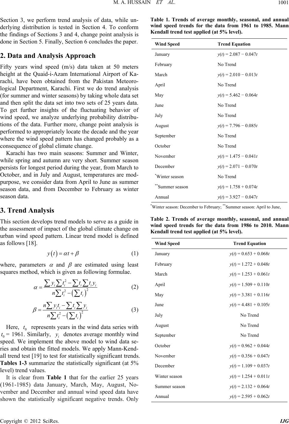

M. A. HUSSAIN ET AL. 1001
Section 3, we perform trend analysis of data, while un-
derlying distribution is tested in Section 4. To conform
the findings of Sections 3 and 4, change point analysis is
done in Section 5. Finally, Section 6 concludes the paper.
2. Data and Analysis Approach
Fifty years wind speed (m/s) data taken at 50 meters
height at the Quaid-i-Azam International Airport of Ka-
rachi, have been obtained from the Pakistan Meteoro-
logical Department, Karachi. First we do trend analysis
(for summer and winter seasons) by taking whole data set
and then split the data set into two sets of 25 years data.
To get further insights of the fluctuating behavior of
wind speed, we analyze underlying probability distribu-
tions of the data. Further more, change point analysis is
performed to appropriately locate the decade and the year
where the wind speed pattern has changed probably as a
consequence of global climate change.
Karachi has two main seasons: Summer and Winter,
while spring and autumn are very short. Summer season
persists for longest period during the year, from March to
October, and in July and August, temperatures are mod-
purpose, we consider data from April to June as summer
season data, and from December to February as winter
season data.
3. Trend Analysis
This section develops trend models to serve as a guide in
the assessment of impact of the global climate change on
urban wind speed pattern. Linear trend model is defined
as follows [18].

yt t

 

(1)
where, parameters  and  are estimated using least
squares method, which is given as following formulae.
2
2
ii
yt
nt


2
iii
ii
tty
t





(2)
2
2
iii i
ii
tt y
t




t
t y
ny
nt
  (3)
Here, 0 represents years in the wind data series with
0= 1961. Similarly, i denotes average monthly wind
speed. We implement the above model to wind data se-
ries and obtain the fitted models. We apply Mann-Kend-
all trend test [19] to test for statistically significant trends.
Tables 1-3 summarize the statistically significant (at 5%
level) trend values.
It is clear from Table 1 that for the earlier 25 years
(1961-1985) data January, March, May, August, No-
vember and December and annual wind speed data have
shown the statistically significant negative trends. Only
Table 1. Trends of average monthly, seasonal, and annual
wind speed trends for the data from 1961 to 1985. Mann
Kendall trend test applied (at 5% level).
Wind Speed Trend Equation
January y(t) = 2.087 − 0.047t
February No Trend
March y(t) = 2.010 − 0.013t
April No Trend
May y(t) = 5.462 − 0.064t
June No Trend
July No Trend
August y(t) = 7.796 − 0.085t
September No Trend
October No Trend
November y(t) = 1.475 − 0.041t
December y(t) = 2.071 − 0.070t
*Winter season No Trend
**Summer season y(t) = 1.758 + 0.074t
Annual y(t) = 3.927 − 0.047t
*Winter season: December to February; **Summer season: April to June,
Table 2. Trends of average monthly, seasonal, and annual
wind speed trends for the data from 1986 to 2010. Mann
Kendall trend test applied (at 5% level).
Wind Speed Trend Equation
January y(t) = 0.653 + 0.068t
February y(t) = 1.272 + 0.048t
March y(t) = 1.253 + 0.061t
April y(t) = 1.509 + 0.110t
May y(t) = 3.381 + 0.116t
June y(t) = 4.481 + 0.105t
July No Trend
August No Trend
September No Trend
October y(t) = 0.962 + 0.044t
November y(t) = 0.356 + 0.047t
December y(t) = 1.109 + 0.037t
Winter season y(t) = 1.254 + 0.011t
Summer season y(t) = 2.132 + 0.064t
Annual y(t) = 2.595 + 0.062t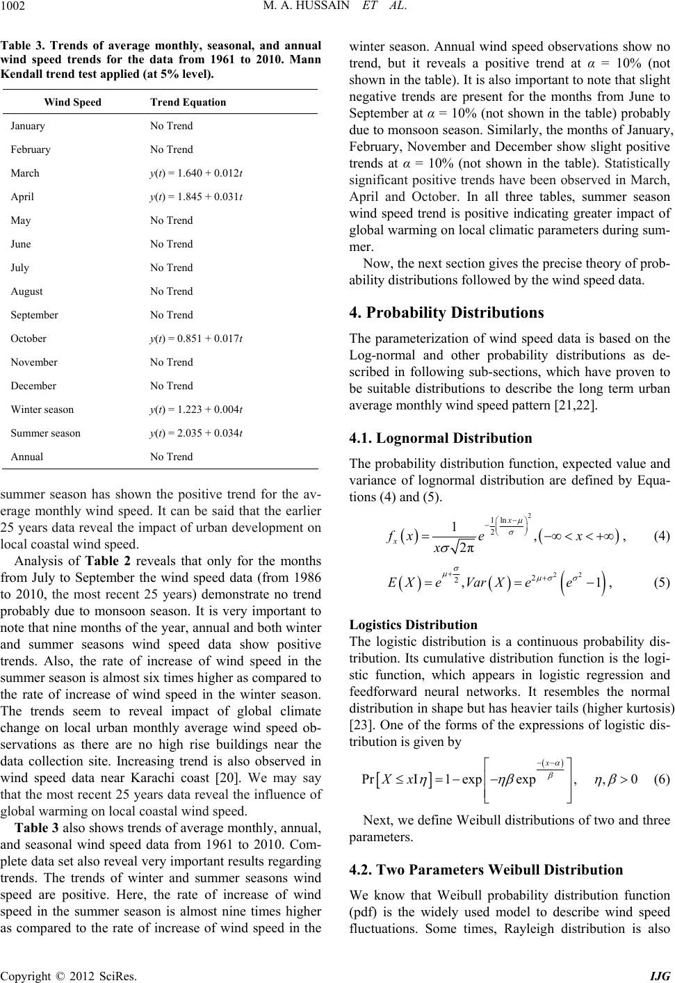

M. A. HUSSAIN ET AL. 1002
Table 3. Trends of average monthly, seasonal, and annual
wind speed trends for the data from 1961 to 2010. Mann
Kendall trend test applied (at 5% level).
Wind Speed Trend Equation
January No Trend
February No Trend
March y(t) = 1.640 + 0.012t
April y(t) = 1.845 + 0.031t
May No Trend
June No Trend
July No Trend
August No Trend
September No Trend
October y(t) = 0.851 + 0.017t
November No Trend
December No Trend
Winter season y(t) = 1.223 + 0.004t
Summer season y(t) = 2.035 + 0.034t
Annual No Trend
summer season has shown the positive trend for the av-
erage monthly wind speed. It can be said that the earlier
25 years data reveal the impact of urban development on
local coastal wind speed.
Analysis of Table 2 reveals that only for the months
from July to September the wind speed data (from 1986
to 2010, the most recent 25 years) demonstrate no trend
probably due to monsoon season. It is very important to
note that nine months of the year, annual and both winter
and summer seasons wind speed data show positive
trends. Also, the rate of increase of wind speed in the
summer season is almost six times higher as compared to
the rate of increase of wind speed in the winter season.
The trends seem to reveal impact of global climate
change on local urban monthly average wind speed ob-
servations as there are no high rise buildings near the
data collection site. Increasing trend is also observed in
wind speed data near Karachi coast [20]. We may say
that the most recent 25 years data reveal the influence of
global warming on local coastal wind speed.
Table 3 also shows trends of average monthly, annual,
and seasonal wind speed data from 1961 to 2010. Com-
plete data set also reveal very important results regarding
trends. The trends of winter and summer seasons wind
speed are positive. Here, the rate of increase of wind
speed in the summer season is almost nine times higher
as compared to the rate of increase of wind speed in the
winter season. Annual wind speed observations show no
trend, but it reveals a positive trend at α = 10% (not
shown in the table). It is also important to note that slight
negative trends are present for the months from June to
September at α = 10% (not shown in the table) probably
due to monsoon season. Similarly, the months of January,
February, November and December show slight positive
trends at α = 10% (not shown in the table). Statistically
significant positive trends have been observed in March,
April and October. In all three tables, summer season
wind speed trend is positive indicating greater impact of
global warming on local climatic parameters during sum-
mer.
Now, the next section gives the precise theory of prob-
ability distributions followed by the wind speed data.
4. Probability Distributions
The parameterization of wind speed data is based on the
Log-normal and other probability distributions as de-
scribed in following sub-sections, which have proven to
be suitable distributions to describe the long term urban
average monthly wind speed pattern [21,22].
4.1. Lognormal Distribution
The probability distribution function, expected value and
variance of lognormal distribution are defined by Equa-
tions (4) and (5).
 
2
1ln
2
1,
2π
x
x
fx ex
x



 

 , (4)

  
 

22
2
2,1EX eVarX ee

 




, (5)
Logistics Distribution
The logistic distribution is a continuous probability dis-
tribution. Its cumulative distribution function is the logi-
stic function, which appears in logistic regression and
feedforward neural networks. It resembles the normal
distribution in shape but has heavier tails (higher kurtosis)
[23]. One of the forms of the expressions of logistic dis-
tribution is given by
Pr1expexp, ,0
x
Xx


 




 


(6)
Next, we define Weibull distributions of two and three
parameters.
4.2. Two Parameters Weibull Distribution
We know that Weibull probability distribution function
(pdf) is the widely used model to describe wind speed
fluctuations. Some times, Rayleigh distribution is also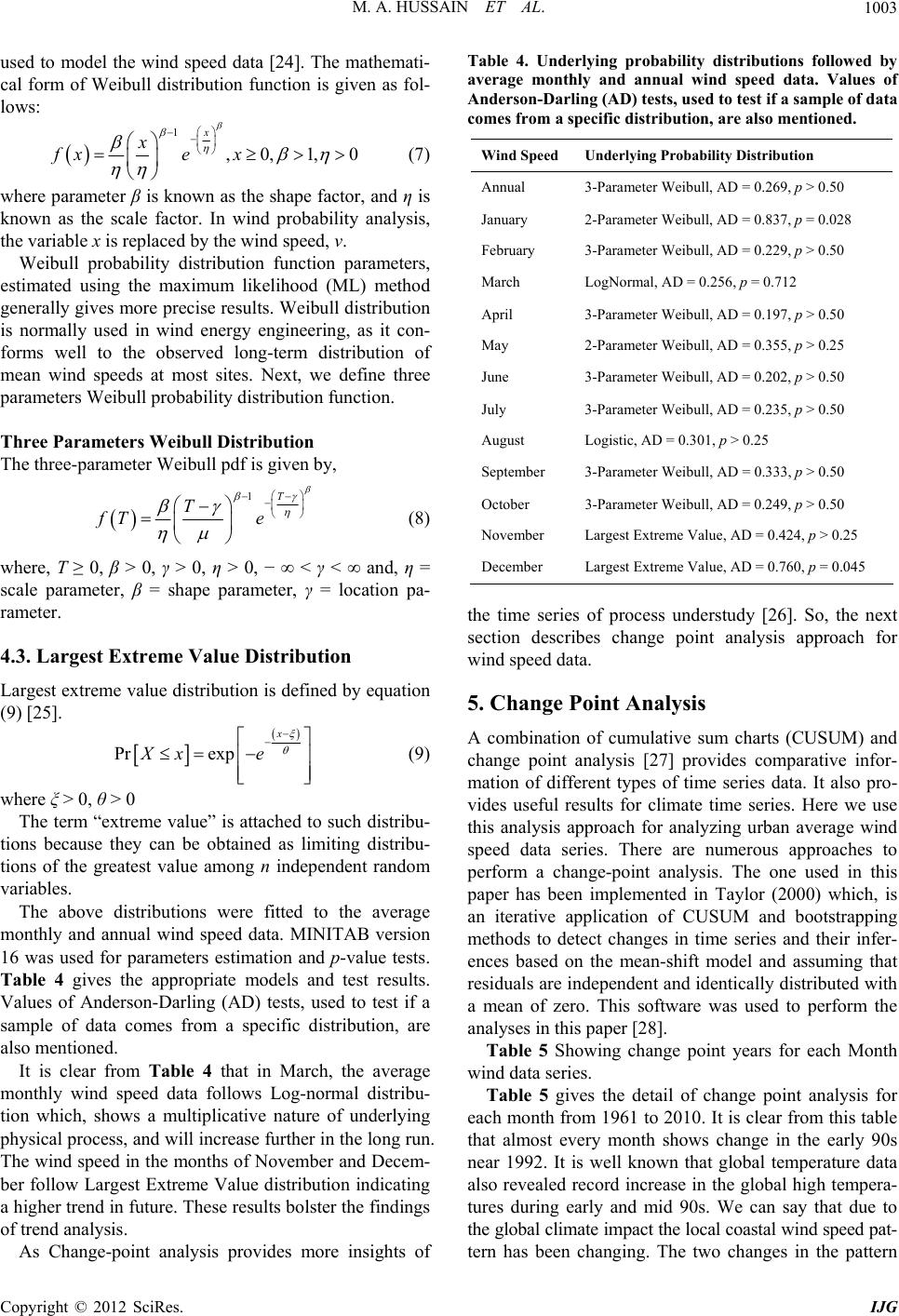

M. A. HUSSAIN ET AL. 1003
used to model the wind speed data [24]. The mathemati-
cal form of Weibull distribution function is given as fol-
lows:

1x
x
fxe x





 




 ,0,1,0
 

(7)
where parameter β is known as the shape factor, and η is
known as the scale factor. In wind probability analysis,
the variable x is replaced by the wind speed, v.
Weibull probability distribution function parameters,
estimated using the maximum likelihood (ML) method
generally gives more precise results. Weibull distribution
is normally used in wind energy engineering, as it con-
forms well to the observed long-term distribution of
mean wind speeds at most sites. Next, we define three
parameters Weibull probability distribution function.
Three Parameters Weibull Distribution
The three-parameter Weibull pdf is given by,

1T
e
T
fT














 (8)
where, T ≥ 0, β > 0, γ > 0, η > 0, − ∞ < γ < ∞ and, η =
scale parameter, β = shape parameter, γ = location pa-
rameter.
4.3. Largest Extreme Value Distribution
Largest extreme value distribution is defined by equation
(9) [25].

Pr eXx xp
x
e













(9)
where ξ > 0, θ > 0
The term “extreme value” is attached to such distribu-
tions because they can be obtained as limiting distribu-
tions of the greatest value among n independent random
variables.
The above distributions were fitted to the average
monthly and annual wind speed data. MINITAB version
16 was used for parameters estimation and p-value tests.
Table 4 gives the appropriate models and test results.
Values of Anderson-Darling (AD) tests, used to test if a
sample of data comes from a specific distribution, are
also mentioned.
It is clear from Table 4 that in March, the average
monthly wind speed data follows Log-normal distribu-
tion which, shows a multiplicative nature of underlying
physical process, and will increase further in the long run.
The wind speed in the months of November and Decem-
ber follow Largest Extreme Value distribution indicating
a higher trend in future. These results bolster the findings
of trend analysis.
As Change-point analysis provides more insights of
Table 4. Underlying probability distributions followed by
average monthly and annual wind speed data. Values of
Anderson-Darling (AD) tests, used to test if a sample of data
comes from a specific distribution, are also mentioned.
Wind Speed Underlying Probability Distribution
Annual 3-Parameter Weibull, AD = 0.269, p > 0.50
January 2-Parameter Weibull, AD = 0.837, p = 0.028
February 3-Parameter Weibull, AD = 0.229, p > 0.50
March LogNormal, AD = 0.256, p = 0.712
April 3-Parameter Weibull, AD = 0.197, p > 0.50
May 2-Parameter Weibull, AD = 0.355, p > 0.25
June 3-Parameter Weibull, AD = 0.202, p > 0.50
July 3-Parameter Weibull, AD = 0.235, p > 0.50
August Logistic, AD = 0.301, p > 0.25
September 3-Parameter Weibull, AD = 0.333, p > 0.50
October 3-Parameter Weibull, AD = 0.249, p > 0.50
November Largest Extreme Value, AD = 0.424, p > 0.25
December Largest Extreme Value, AD = 0.760, p = 0.045
the time series of process understudy [26]. So, the next
section describes change point analysis approach for
wind speed data.
5. Change Point Analysis
A combination of cumulative sum charts (CUSUM) and
change point analysis [27] provides comparative infor-
mation of different types of time series data. It also pro-
vides useful results for climate time series. Here we use
this analysis approach for analyzing urban average wind
speed data series. There are numerous approaches to
perform a change-point analysis. The one used in this
paper has been implemented in Taylor (2000) which, is
an iterative application of CUSUM and bootstrapping
methods to detect changes in time series and their infer-
ences based on the mean-shift model and assuming that
residuals are independent and identically distributed with
a mean of zero. This software was used to perform the
analyses in this paper [28].
Table 5 Showing change point years for each Month
wind data series.
Table 5 gives the detail of change point analysis for
each month from 1961 to 2010. It is clear from this table
that almost every month shows change in the early 90s
near 1992. It is well known that global temperature data
also revealed record increase in the global high tempera-
tures during early and mid 90s. We can say that due to
the global climate impact the local coastal wind speed pat-
tern has been changing. The wo changes in the pattern t

M. A. HUSSAIN ET AL. 1004
Table 5. Change point analysis for month wind speed data from 1961 to 2010.
Urban Average Monthly Wind Speed Series (1961-2010 ) Change Point Analysis Summary
Year Jan Feb Mar Apr May Jun Jul Aug Sep Oct Nov Dec
1972 Y Y
1974
1977 Y Y Y Y Y
1980
1981 Y
1982
1983
1984
1985 Y
1986
1987
1992 Y Y Y Y Y Y Y Y
1995 Y Y
1999 Y Y
2001
2005
2009
Years 2 1 1 3 2 2 2 2 1 1 2 2
of wind speed data (1961-2010) in the month of January,
as depicted in Figure 1(a), are represented by the shifts
in the shaded background. The shaded background repre-
sents a region expected to contain all the values based on
the current model that two changes occurred. Similar
changes can be observed in all figures for the remaining
months of the year. Thus, change point analysis reveals
that it the most recent 25 years where the wind speed
changed its pattern.
Following graphs Figures 1(a)-(l) show graphical
presentation of the results of the change-point analysis of
the monthly urban wind speed data series.
6. Results and Discussion
Three methods were conducted to investigate the impact
of global climate change on the fluctuating pattern of
average urban wind speed. Trend analysis revealed that
for the earlier 25 years (1961-1985) data January, March,
May, August, November and December and annual wind
speed data have shown the statistically significant nega-
tive trends. But, summer season has shown the positive
trend for wind speed. Similarly, the most recent 25 years
demonstrate no trend for the months from July to Sep-
tember the wind speed data due to the monsoon season.
In this era, nine months of the year, annual and both
winter and summer seasons wind speed data have shown
positive trends. Also, the rate of increase of wind speed
in the summer season is almost six times higher as com-
pared to the rate of increase of wind speed in the winter
season. The trends seem to reveal impact of global cli-
mate change on local urban monthly average wind speed
observations as there are no high rise buildings near the
data collection site. So, the most recent 25 years data
revealed the influence of global warming on local coastal
wind speed.
Table 3 has demonstrated the trends of average
monthly, annual, and seasonal wind speed for the com-
plete data set. It revealed very important results regarding
trends. The trends of winter and summer seasons wind
speed are positive. Here, the rate of increase of wind
speed in the summer season is almost nine times higher
as compared to the rate of increase of wind speed in the
winter season. But, annual wind speed observations show
no trend. Significant positive trends have been observed
in March, April and October. In the three data sets,
summer season wind speed trend is positive indicating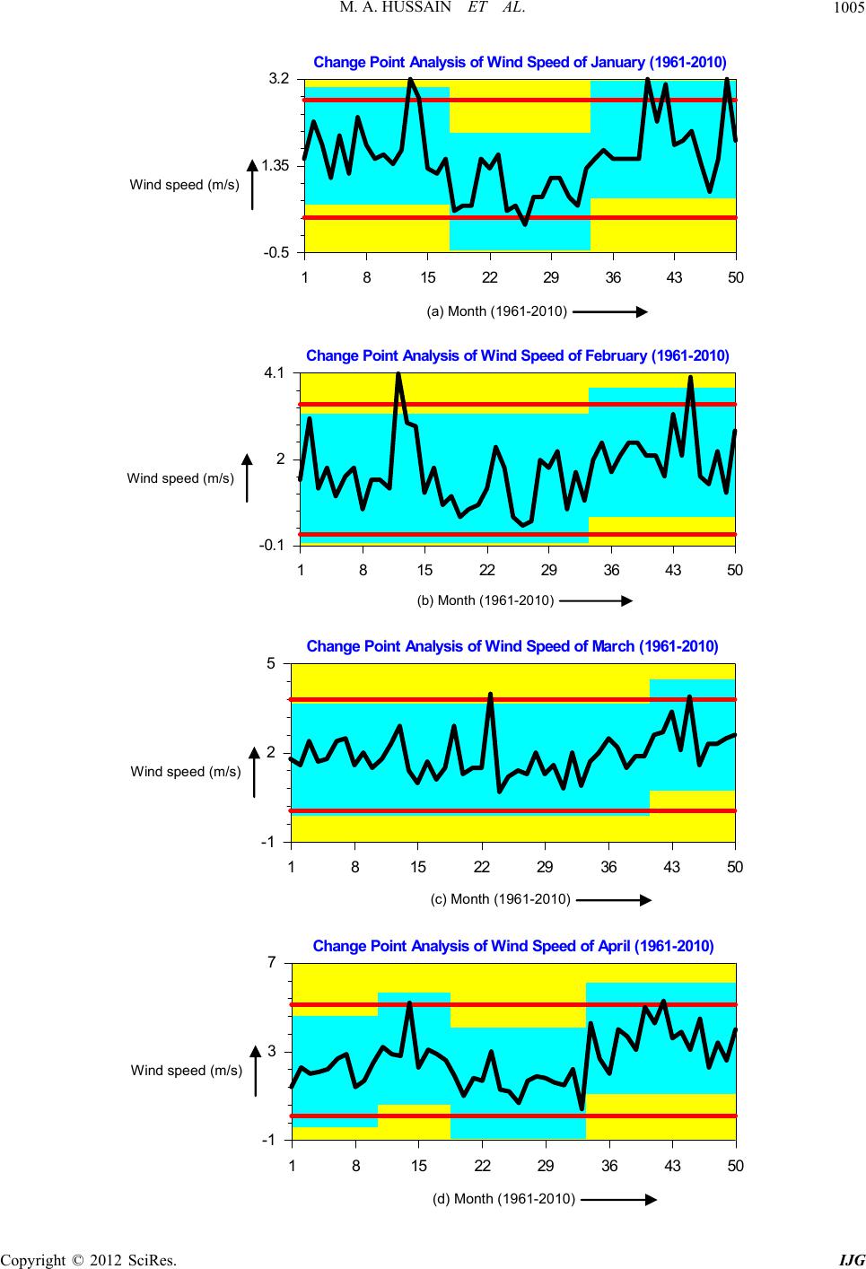

M. A. HUSSAIN ET AL. 1005
Change Point Analysis of Wind Speed of January
3.2
1.35
-0.5
1815 2229 36
(1961-2010)
43 5
0
Wind speed (m/s)
(a) Month (1961-2010)
Change Point Analy sis of Wind Speed of February
4.1
2
-0.1
18152229 36
(1961-2010)
43 50
Wind speed (m/s)
(b) Month (1961- 20 10)
Change Point Analysis of Wind Speed of March (
5
2
-1
18152229 36
1961-2010)
43 5
0
Wind speed (m/s)
(c) Month (196 1- 20 10)
Change Point Analysis of Wind Speed of April (
7
3
-1
181522 29 36
1961-2010)
43 5
0
Wind speed (m/s)
(d) Month (1961- 2010 )

M. A. HUSSAIN ET AL. 1006
Change Point Analysis of Wind Speed of May (
12
5
-2
181522 29 36
1961-2010)
43 50
Wind speed (m/s)
(e) Month (19 61- 20 10 )
Change Point Analysis of W in d Speed of June (
11
5
-1
181522 2936
1961-2010)
43 50
Wind speed (m/s)
(f) Mont h (196 1- 2010)
Change Point Analysis of Wind Speed of July (1
12
6
0
1815 2229 36
961-2010)
43 50
Wind speed (m/s)
(g) Month (19 6 1- 20 1 0 )
Change Point Analysis of Wind Speed of August
11
6.5
2
1815 2229 36
(1961-2010)
43 5
0
Wind speed (m/s)
(h) Mont h (1961- 20 10 )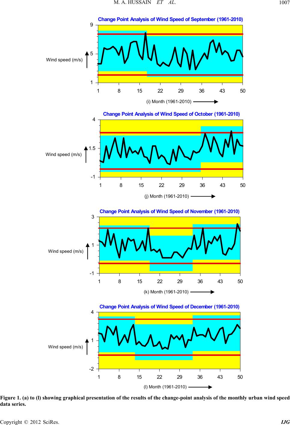

M. A. HUSSAIN ET AL. 1007
Change Point Analysis of Wind Speed of September
9
5
1
1815 22 29 36
(1961-2010)
43 50
Wind speed (m/s)
(i) Mont h (1 961-20 1 0)
Change Point Analysis of Wind Speed of October
4
1.5
-1
18152229 36
(1961-2010)
43 50
Wind speed (m/s)
(j) Month (1961-201 0)
Change Point Analysis of Wind Speed of November
3
1
-1
18152229 36
(1961-2010)
43 50
Wind speed ( m/s )
(k) Month (1961- 2010)
Change Point Analysis of Wind Speed of Decembe
4
1
-2
1815 2229 36
r (1961-2010)
43 50
Wind speed (m/s)
(l) Month (196 1-2 010)
Figure 1. (a) to (l) showing graphical presentation of the results of the change-point analysis of the monthly urban w ind spee d
ata series. d

M. A. HUSSAIN ET AL. 1008
impact of global warming on local climatic parameters
during summer.
If different probability distribution functions were
fitted to wind speed data, it revealed that in the month of
March, the average monthly wind speed data followed
Log-normal distribution showing a multiplicative nature
of underlying physical process, whereas the wind speed
in the months of November and December followed
Largest Extreme Value distribution indicating that it
would show higher trends.
Results of the change point analysis (see Figures 1(a)-
(l)) have been summarized in Table 5. It is clear from
this table that almost every month shows change in the
early 90s near 1992. We can say that due to the global
climate impact the local coastal wind speed pattern has
been changing. The two changes in the pattern of wind
speed data (1961-2010) in the month of January, as de-
picted in Figure 1(a), are represented by the shifts in the
shaded background. The analysis performed by change
point analysis has also confirmed that wind speed pattern
has changed in the most recent 25 years. The trends and
underlying probability distribution models of urban wind
speed data cannot predict specific events but for some
types of extremes they can indicate how the urban wind
speed profiles are likely to change in the future.
7. Conclusions and Future Outlook
As discussed in Section 1, the effects of global warming
and climate change is complex in nature and not com-
pletely understood. However, the urban wind data series
show different fluctuating pattern in three wind series
data. The wind series data during 1986 and 2010, the
most recent era, depict significant positive trends proba-
bly because of the consequences of global climate
change, and is also important in indicating the possible
future wind fluctuations in the area under study. Under-
lying distributions of wind speed also revealed the over-
all increasing trends both in annual and monthly wind
speed fluctuations. Change point analysis of wind data
confirmed that some change in fluctuating pattern of
physical process has taken place in the most recent era.
Analysis performed on urban wind speed pattern showed
that somewhere in 1992 the wind speed pattern changed
its speed probably due to global climate impact.
Finally, we can say that in the vicinity of Karachi, it
appeared to increase the average wind speed pattern due
to changes in global climate as the city of Karachi is lo-
cated at the coast of Arabian Sea. Methods and tech-
niques employed to study local wind speed fluctuations
phenomenon has provided an increase in the skills and
knowledge necessary to deal with possible future local
and global climate change. In the future, knowledge of
urban climate change will be of importance for the resi-
dents of mega cities. Larger cities will likely emphasize
the climatic effects, especially if the urban growth occurs
at present pace. The knowledge and understanding about
these important climatic factors would help us in fore-
casting the future direction of wind pattern dynamics,
which will help in mitigation of consequences of both
local and global climate change in future.
8. Acknowledgements
We thank Pakistan Meteorological Department, Karachi,
for providing us urban wind speed, and tropical cyclone
data.
REFERENCES
[1] M. A. Hussain, “Mathematical Aspects of The Impact of
Urban Greenhouse Gas Emissions on Global Warming,”
Ph.D. Thesis, Federal Urdu University of Arts, Science
and Technology, Karachi, 2006.
[2] M. A. Hussain and M. R. K. Ansari, “Some Insights of
Local and Global Temperatures Dynamics,” Arabian
Journal for Science and Engineering, Vol. 35, No. 1A,
2010, pp. 103-113.
[3] M. A. Hussain and M. R. K. Ansari, “Statistical Aspects
of Global Warming Dynamics,” Arabian Journal for
Science and Engineering, Vol. 32, No. 2A, 2007, pp. 189-
201.
[4] M. A. K. Yousuf Zai, M. A. K. Ansar, J. Quamar, J. Iqbal
and M. A. Hussain, “Predicting the Variations in the Wa-
velength Structures of the Incoming Radiation Due to
Ozone Layer Depletion at Arabian Sea,” The Nucleus,
Vol. 45, No. 1, 2008, 7 p.
[5] M. A. K. Yousuf Zai, M. A. K. Ansari, J. Quamar, J.
Iqbal and M. A. Hussain, “Comparison of AR Strategy
with that of Regression Approach for Determining Ozone
Layer Depletion as a Physical Process,” The Nucleus, Vol.
45, No. 2, 2008, 7 p.
[6] R. Meldensohn, et al., “The Impact of Climate Change on
Global Tropical Cyclone Damage,” Nature Climate
Change, Vol. 2, No. 10, 2012, pp. 205-209.
doi:10.1038/nclimate1357
[7] M. A. Hussain, et al., “Persistency Analysis of Cyclone
History in Arabian Sea,” The Nucleus, Vol. 48, No. 4,
2011, pp. 273-277.
[8] M. A. Hussain, et al., “Forecast Models for Urban Ex-
treme Temperatures: Karachi Region as a Case Study,”
The Nucleus, Vol. 47, No. 4, 2010, pp. 301-311.
[9] M. A. Hussain, et al., “Arabian Seawater Temperature
Fluctuations in the Twentieth Century,” Journal of Basic
and Appliewd Sciences, Vol. 8, No. 1, 2012, pp. 105-109.
doi:10.6000/1927-5129.2012.08.01.24
[10] S. H. L. Yim, J. C. H. Fung, and A. K. H. Lau, “Meso-
scale Simulation of Year-to-Year Variation of Wind
Power Potential over Southern China,” Energies, Vol. 2,
2009, pp. 340-361. doi:10.3390/en20200340
[11] J. M. Dryden, “Potential Climate Change Impacts on
Wind Resources in Oklahoma: A Focus on Future Energy

M. A. HUSSAIN ET AL. 1009
Output,” Masters Thesis, The University of Oklahoma,
Norman, 2008.
[12] Ministry of Petroleum & Natural Resources, Hydrocarbon
Development Institute of Pakistan, “Pakistan Energy Year
Book,” 2004.
[13] www.urckarachi.org/IEE_Study_of_DHA-WFD_Project_
(ii).pdf
[14] S.-H. Lee and H.-D. Kim, “Effects of Regional Warming
Due to Urbanization on Daytime Local Circulations in a
Complex Basin of the Daegu Metropolitan Area, Korea,”
Journal of Applied Meteorology and Climatology, Vol. 47,
No. 5, 2008, pp. 1427-1441. doi:10.1175/JAMC1504.1
[15] ftp://ftp1.esrl.noaa.gov/users/.../Liu&Curry_manu_r1%20
1.doc
[16] http://www.globalchange.gov/images/cir/pdf/National.pdf
[17] S. Qureshi, “The Fast Growing Megacity Karachi as a
Frontier of Environmental Challenges: Urbanization and
Contemporary Urbanism Issues,” Journal of Geography
and Regional Planning, Vol. 3, No. 11, 2010, pp. 306-
321.
[18] M. A. Hussain, et al., “Arabian Seawater Temperature
Fluctuations in the Twentieth Century,” Journal of Basic
and Applied Sciences, Vol. 8, No. 1, 2012, pp. 105-109.
doi:10.6000/1927-5129.2012.08.01.24
[19] S. D. Río, A. Cano-Ortiz, L. Herrero and A. Penas, “Re-
cent Trends in Mean Maximum and Minimum Air Tem-
peratures over Spain (1961-2006),” Theoretical and Ap-
plied Climatology, Vol. 109, No. 3-4, 2012, pp. 605-626.
doi:10.1007/s00704-012-0593-2
[20] M. A. Hussain, S. Abbas and M. R. K. Ansari, “Wind
Speed Analysis of Some Coastal Areas near Karachi,”
Pakistan Academy of Sciences, 2012.
[21] F. A. L. Jowder, “Weibull and Rayleigh Distribution
Functions of Wind Speeds in Kingdom of Bahrain,” Wind
Engineering, Vol. 30, No. 5, 2006, pp. 439-445.
doi:10.1260/030952406779502650
[22] H. Basumatary, et al., “Weibull Parameter Estimation: A
Comparison of Different Methods,” Wind Engineering,
Vol. 29, No. 3, 2005, pp. 309-316.
doi:10.1260/030952405774354895
[23] http://en.wikipedia.org/wiki/Logistic_distribution
[24] J. V. Seguro and T. W. Lambert, “Modern Estimation of
the Parameters of the Weibull Wind Speed Distribution
for Wind Energy Analysis,” Journal of Wind Engineering
and Industrial Aerodynamics, Vol. 85, No. 1, 2000, pp.
75-84. doi:10.1016/S0167-6105(99)00122-1
[25] N. L. Johnson, S. Kotz and N. Balakrishnan, “Continuous
Univariate Distributions,” John Wiley, New York, 2004.
[26] Reeves, Jaxk, J. Chen, X. L. Wang, R. Lund and Q. Q. Lu,
“A Review and Comparison of Changepoint Detection
Techniques for Climate Data,” Journal of Applied Mete-
orology and Climatology, Vol. 46, No. 6, 2007, pp. 900-
915. doi:10.1175/JAM2493.1
[27] W. A. Taylor, “Change-Point Analyzer 2.0 Shareware
program,” Taylor Enterprises, Libertyville, 2000.
http://www.variation.com/cpa/tech/changepoint.html