A Systematization for One-Loop 4D Feynman Integrals-Different Species of Massive Fields

doi:10.4236/jmp.2012.310178

Journal of Modern Physics, 2012, 3, 1408-1449

http://dx.doi.org/10.4236/jmp.2012.310178 Published Online October 2012 (http://www.SciRP.org/journal/jmp)

A Systematization for One-Loop 4D Feynman

Integrals-Different Species of Massive Fields

O. A. Battistel1, G. Dallabona2

1Departamento de Fsica, Universidade Federal de Santa Maria, Santa Maria, Brazil

2Departamento de Ciências Exatas, Universidade Federal de Lavras, Lavras, Brazil

Email: orimar.battistel@gmail.com, gilson.dallabona@gmail.com

Received August 20, 2012; revised September 20, 2012; accepted October 2, 2012

ABSTRACT

A systematization for the manipulations and calculations involving divergent (or not) Feynman integrals, typical of the

one loop perturbative solutions of Quantum Field Theory, is proposed. A previous work on the same issue is general-

ized to treat theories and models having different species of massive fields. An improvement on the strategy is adopted

so that no regularization needs to be used. The final results produced, however, can be converted into the ones of rea-

sonable regularizations, especially those belonging to the dimensional regularization (in situations where the method

applies). Through an adequate interpretation of the Feynman rules and a convenient representation for involved propa-

gators, the finite and divergent parts are separated before the introduction of the integration in the loop momentum. On-

ly the finite integrals obtained are in fact integrated. The divergent content of the amplitudes are written as a combina-

tion of standard mathematical object which are never really integrated. Only very general scale properties of such ob-

jects are used. The finite parts, on the other hand, are written in terms of basic functions conveniently introduced. The

scale properties of such functions relate them to a well defined way to the basic divergent objects providing simple and

transparent connection between both parts in the assintotic regime. All the arbitrariness involved in this type of calcula-

tions are preserved in the intermediary steps allowing the identification of universal properties for the divergent inte-

grals, which are required for the maintenance of fundamental symmetries like translational invariance and scale inde-

pendence in the perturbative amplitudes. Once these consistency relations are imposed no other symmetry is violated in

perturbative calculations neither ambiguous terms survive at any theory or model formulated at any space-time dimen-

sion including nonrenormalizable cases. Representative examples of perturbative amplitudes involving different species

of massive fermions are considered as examples. The referred amplitudes are calculated in detail within the context of

the presented strategy (and systematization) and their relations among other Green functions are explicitly verified. At

the end a generalization for the finite functions is presented.

Keywords: Feynman Integrals; Perturbative Amplitudes

1. Introduction

Given the fact that exact solutions for Quantum Field

Theories (QFT) are rarely possible, almost all knowledge

constructed through this formalism about the phenome-

nology of fundamental interacting particles has been ob-

tained within the context of perturbative techniques. In

order to get the predictions in such framework, many

nontrivial mathematical difficulties must be circum-

vented due to the presence of infinities or divergences in

the perturbative series for the elementary process. We

have to find a consistent prescription to handle the ma-

thematical indefiniteness involved, which means to avoid

the breaking of global and local symmetries as well as

simultaneously to avoid ambiguities in the produced re-

sults. By ambiguities we understand any dependence on

the final results on possible arbitrary choices involved

in intermediary steps of the calculations. If they exist,

undoubtedly, the predictive power of the formalism it is

destroyed. The first and most immediate of such ambi-

guities are those associated with the choices of the labels

for the momenta carried by the internal lines of loop per-

turbative amplitudes. They naturally appear when the

divergence degree is higher than the logarithmic one. The

result for such amplitudes may be dependent on the par-

ticular choices for the routings due to the fact that in this

case the amplitudes are not invariant under shifts in the

loop momentum. A second and important type of choice

is the regularization prescription. Two different choices

for the regularization can lead to different results for the

calculated amplitudes. These two kinds of ambiguities

are very well-known in the corresponding literature. A

third and more general one has been recently considered

C

O. A. BATTISTEL, G. DALLABONA 1409

in the context of perturbative calculations, which is the

denominated scale ambiguities [1]. They are related to

the choice for a common scale for the finite and diver-

gent parts when they are separated in a Feynman integral.

There is an arbitrariness involved in the separation of

these terms in a summation when they have different

divergence degrees. The scale properties of the pertur-

bative amplitudes are the most general guides for the

consistency of the procedures. There are situations in

which a symmetry violating is non-ambiguous relative to

the choice for the labels of the internal lines momentum

but it is ambiguous relative to the choice for the common

scale. In addition to the difficulties coming from the di-

vergences we frequently have also those coming from the

extension of the mathematical expressions involved. Apart

from a few number of simple amplitudes, the mathe-

matical complexity of the obtained expression, not rarely,

makes prohibitive any analysis of the obtained results.

Considering these aspects of the perturbative calcula-

tions in QFT it would be desirable to get a procedure to

manipulate and calculate divergent physical amplitudes

without compromising the results with a particular regu-

larization scheme. In addition to this, we would like to

make the calculations preserving all the possible choices

for the arbitrariness involved like those related to the

choice of routings for the internal momenta and for the

common scale for the finite and divergent parts. To com-

plete such adequate calculational strategy it would be

desirable to get also a systematization for the finite parts

of the amplitudes in a way that the mathematical expres-

sions become simple allowing the required analysis and

algebraic operations related to the renormalization pro-

cedures, among others.

If one agrees with this line of reasoning the present

work may constitute a contribution on this direction. We

present in this paper a calculational strategy which ful-

fills the requirements stated above. We start by formu-

lating the steps involved in the calculation of perturbative

amplitudes, through the corresponding Feynman rules, in

such a way that no regularization needs to be specified.

The calculations are made by using arbitrary choices for

the internal lines of loop amplitudes and an arbitrary

scale parameter is introduced in the separation of terms

associated with different degrees of divergences. Through

the procedure no divergent integral is really calculated.

They are reduced to standard forms which are then un-

touched. The finite parts are not contaminated with any

type of modification and a systematization through

structure functions is introduced. The result is a com-

pletely algebraic procedure where no limits or expan-

sions are taken. All the procedures like Ward identities

verifications, renormalization procedures and so on, are

made by using properties of the finite functions and basic

divergent objects. In addition to this, the important aspect

of the procedure is its general character; all the ampli-

tudes in all theories and models are treated in an abso-

lutely identical way. We treat amplitudes in renormaliz-

able and non renormalizable theories formulated in even

and odd space-time dimension within the same strategy.

Symmetry violating terms as well as ambiguous ones

may be simultaneously eliminated in a consistent way.

Anomalous amplitudes are consistently described with-

out the presence of ambiguities in any (even) space-time

dimension.

The material we present in this work may be consid-

ered as an extension of that presented in [2]. The ques-

tions considered here are not new. In the literature there

are many works about this issue and certainly many oth-

ers continue to be done nowadays. In particular, the re-

duction of tensor integrals to scalar ones, made in the

present work through the properties of the introduced

finite functions, has been studied by Passarino and Velt-

man [3] as well as other authors [4-12]. The scalar inte-

grals has been considered by G.’t Hooft and Veltman

[13]. Recently, new works have been produced specially

involving massless propagators like in [14-29] (and ref-

erences therein). The present systematization for the per-

turbative calculations must be understood as a contribu-

tion to this type of investigation. The very general char-

acter of the procedure and the absence of restrictions of

applicability may represent some advantages which can

be useful for some users of the perturbative solutions of

QFT’s. With the material presented here any self-energy,

decay amplitude and elastic scattering of two fields can

be calculated in fundamental theories.

The work is organized as follows. In the Section 2 we

define the set of basic one-loop 4D Feynman integrals

which we will discuss in future sections. In the Section 3

we explain the strategy adopted to handle the diver-

gences as well as we define the basic divergent objects

used to write the divergent content of the perturbative

amplitudes. The basic functions (and some of their useful

properties) used to systematize the finite parts of the am-

plitudes are introduced in the Section 4. The solution of

the basic one-loop integrals is considered in the Section 5

and the explicit calculation of perturbative amplitudes in

the Section 6. In the Section 7 we consider the explicit

verification of the relations among the Green functions

for the calculated amplitudes and in the Section 8 the

questions related to the ambiguities and symmetry rela-

tions are discussed. A generalization for the finite func-

tions and their useful properties are presented in the Sec-

tion 9 and, finally, in the Section 10 we present our final

remarks and conclusions.

2. Basic One-Loop Feynman Integrals

First of all we call the attention to the fact that in pertur-

O. A. BATTISTEL, G. DALLABONA

1410

bative calculations, independently of the specific theory

or model, in loop amplitudes, we have to take the inte-

gration over the unrestricted momentum. We can con-

sider such an operation as the last Feynman rule. Pre-

cisely at this step all the one-loop perturbative ampli-

tudes will become combinations of a relatively small

number of mathematical structures, the Feynman inte-

grals. Some of such structures are undefined quantities

because they are divergent integrals. Given this situation

we have at our disposal two distinct but, in principle,

equivalent attitudes to adopt. We can perform the calcu-

lation of the desired amplitudes one by one, within the

context of a chosen regularization prescription or equiva-

lent philosophy, ignoring any type of possible systemati-

zation of the procedures or identifying the set of opera-

tions we have to repeat in calculating different ampli-

tudes considering such required operations in a separat-

edly way. In adopting the second option, the immediate

systematization of the perturbative calculations is to con-

sider the study of the set of Feynman integrals we need to

solve in order to calculate all the one-loop amplitudes.

Here we will restrict our attention to the fundamental

theories but this attitude can always be followed.

In this linere of asoning we first separate the ampli-

tudes by the number of internal lines or propagators.

Thus the one propagator amplitudes in fundamental theo-

ries will be reduced, in some step of the calculations, to a

combination of the integrals



4

1;

d

;.

2πi

k

D





22

ii

km



 





11

II



 (1)

Here we introduced the definition

i

Dk . Such structures are the most sim-

ple ones but are also those having the most severe degree

of divergences: the cubic one 1

I



. The one-loop am-

plitudes having two internal propagators, on the other

hand, will be written as a combination of the structures



4

22 24

d

;;

2π

k

II I





1; ;.

ij

kkk

D



.DDD

(2)

Here ijij The highest degree of divergence

here is the quadratic one occurring in 2

I





. In calculating

amplitudes having three internal propagators we need to

evaluate the integrals







4

33 334

1; ;

d

;; ;;

2πijl

kkkkkk

k

II IID





DDD

.

(3)

Here we have defined ijlij l



. The higher degree

of divergence involved in the above set of integrals is the

linear one in 3

I





. Two of them are finite structures. We

can introduce also the ingredients required to calculate

amplitudes having four internal lines, the four propaga-

tors Feynman integrals







44 444

4

;; ;;

1; ;;;

d.

2πijlm

II III

kkkkkkkkkk

k

D





DDD

(4)

Now ijlmijl m



. Only one of such structures is

divergent which is the logarithmically divergent structure

4

I





kk

k

.

In the above definitions i and i

m are the arbi-

trary momentum carried by an internal propagator and its

mass, respectively. The arbitrary internal momenta i

are related to the external ones through the relations of

energy-momentum conservation in vertices connecting

the internal lines with the external ones. The adoption of

arbitrary routing for the internal lines momenta is of cru-

cial importance due to the divergent character of the

Feynman integrals involved, in particular for those hav-

ing degree of divergence higher than the logarithmic one

just because in this case the result may be dependent on

the chosen routing. In adopting such general arbitrary

routing for the internal lines we can identify possible

ambiguous terms arising in a certain calculation which

are undefined combinations of the internal lines momenta

(not related to the external ones). This aspect will be-

come clear in a moment.

When we find a combination of divergent Feynman

integrals in a certain step of the calculation of a pertur-

bative amplitude, in order to give an additional step we

have to specify the prescription we will adopt to handle

the mathematical indefinitions involved. Usually this

means adopting a regularization prescription or an equiv-

alent philosophy. All the results, after this, will be com-

promised with the particular aspects of the chosen regu-

larization. The so obtained results will represent only the

consequences of the arbitrary choice made for the regu-

larization. Even if there are elements of the calculations

which are independent of the regularization scheme em-

ployed, certainly, there are parts of the result which will

be specific of the particular regularization used.

In the present work we will follow an alternative pro-

cedure. We will not compromise the results with a par-

ticular choice in any step of the calculation. The choice

for the regularization will be avoided. The routing of the

internal lines momenta will be taken as arbitrary and the

most important and new aspect specially for calculations

involving different species of massive fields, the com-

mon scale for the finite and divergent parts, will be as-

sumed also as being arbitrary. With this attitude all the

possibilities for such choices will still remain in the final

results. Thus, it will be possible to make a very general

analysis of the results searching for the universal condi-

O. A. BATTISTEL, G. DALLABONA 1411

tions which are necessary to be preserved in order to get

consistent results in perturbative calculations. This means

to obtain results which are simultaneously free from am-

biguous and symmetry violating terms. In order to fulfill

this program, in the next section, we will describe the

strategy to be adopted in the manipulations and calcula-

tions of divergent Feynman integrals.

3. The Strategy to Handle Divergent

Feynman Integrals and the Basic

Divergent Structures

When we use the Feynman rules to construct the pertur-

bative amplitudes there are two distinct steps. First, with

propagators, vertex operators, combinatorial factors,

traces over Dirac matrices, traces over internal symme-

tries operators and so on, we construct the amplitudes for

one value of the loop momentum k. The next step is to

take a summation over all values for such momentum,

since it is not restricted by the energy momentum con-

servation at all vertices of the corresponding diagram.

This means integrating over the loop momentum. It is

possible to use these two distinct moments of the calcu-

lation to formulate a strategy to handle the divergences

present in perturbative calculation of QFT which may

avoid the use of a regularization [30]. The idea is very

simple and does not involve any kind of magic. Only an

adequate interpretation of the usual procedures is re-

quired. The first step is the same described above: to

construct the amplitude corresponding to one value of the

unrestricted momentum. Then before taking the integra-

tion, the last Feynman rule, we make a counting in the

power of loop momentum in order to get the superficial

degree of divergence of the amplitude in the space-time

dimension we are working. Having this at hand we adopt

the following representation for the involved propagators



















22

1

22

=0

1

22

11

12

iii

j

Nii

j

N

ii

N

Dkk m

kkk

k

kkk

kk





















22

2

1

222

22

,

j

i

N

i

ii

m

km















(5)

taking N in the summation as equal or major than the

superficial degree of divergence. Here



is an arbitrary

parameter having dimension of mass which plays the role

of a common scale to both finite and divergent parts of

the corresponding Feynman integral. Through this pa-

rameter a precise connection between the finite and di-

vergent parts is stated. Note that (as must be required) the

expression above is an identity and in addition the right

hand side is really independent of the arbitrary parameter

2



. After the adoption of the adequate representation for

the propagators and making all the convenient algebraic

reorganizations, we take the integration over the loop

momentum k. Then we note that the internal momenta

dependent parts of the Feynman integrals are located

only in finite integrals. On the other hand, the divergent

parts will reside in standard forms of divergent integrals,

after a convenient reorganization, where no physical pa-

rameter is present. Then we can perform the integration

of the finite integrals obtained and in the divergent ones

we need not to make any additional operation.

In order to allow a compactation of some expressions

in future sections it is convenient to introduce the defini-

tion ii i

222

2i

A

kkk m



 , so that we can write the

above expression as



1

11

22 22

=0

11

1jN

jN

Nii

jN

j

ii

AA

DkkD

















. (6)

The steps above described, required to implement the

procedure, can be formulated within the context of the

language of regularizations. In such formulation we take

the integration over the loop momentum and then the

divergences are stated. We adopt then a regularization in

an implicit way in all Feynman integrals. It is required of

such regularization distribution only very general proper-

ties. In addition to rendering the integral convergent we

require that such distribution is even in the loop momen-

tum in order to be consistent with the Lorentz symmetry

and that a “connection limit” exists. Schematically

  



 

2

44

22

44

4

dd

lim ,

2π2π

d.

2π

ii

i

kk

fkfkG k

kfk





















where the i



s



are parameters of the distribution





22

,Gki, and the limits which allow to remove the

distribution in the finite integrals





2

22

lim, 1,

ii

i

Gk



 

must be well-known. By assuming the presence of this

very general regularization we can manipulate the inte-

grand through algebraic identities just because the inte-

grals are then finite. Next, the identity (5) is used to re-

write the propagators in the Feynman integrals. In the so

obtained finite integrals we take the connection limit

eliminating the regularization and performing then the

integration. In the divergent integrals so obtained no ad-

ditional modifications are made. Only a convenient reor-

ganization in the form of standard objects is promoted.

There are no practical differences in both procedures

O. A. BATTISTEL, G. DALLABONA

1412

described above. The only difference is the presence of

the subscript in the divergent integrals indicating

that a regularization was assumed in an implicit way. The

first formulation however represents the evolution of the

second one proposed and developed by O. A. Battistel

and denominated as implicit regularization, just because

it allows us to perform all the necessary calculations

without mentioning the word regularization in perturbat-

ive calculation for any purposes, as we shall see in what

follows when representative examples of amplitudes

calculations will be considered in detail.



The terms which will be converted in divergent inte-

grals, when the integration over the loop momentum is

taken, can be conveniently organized so that all the di-

vergent content is present in the standard objects (at the

one-loop level in fundamental theories)



4

2

44

22

44

43

22

24

dd

2π2π

4

dd

2π2π

kkkk

k

4

43

22

43

22

4

,

g kk

k

g

kk

k

g kk

k



 



  















□



 





(7)



44

2

43

22

4

d

Δ

2π2π

kk

k









42

22

d

,

g

k









(8)



44

4

22

2d

,

kk g

k











2

42

22

d

2π2π

kk

k







 



 (9)



4

2

42

22

d1

,

k







log2π

I



 (10)



4

2

quad 422

d1k

Ik



.

2π









(11)

In nonrenormalizable theories or in two or more loops

calculations new objects analogous to these can be de-

fined. Note that all the steps performed are perfectly va-

lid within reasonable regularization prescriptions, in-

cluding the dimensional regularization technique. This

means that it is possible to make contact with the results

corresponding to the ones belonging to such methods. To

do this it is only necessary to evaluate the divergent

structures obtained according to the specific chosen re-

gularization prescription just because the finite parts

must be the same due to the fact that, in all acceptable

regularization the connection limit must exist. As a con-

sequence, finite integrals must not be modified. More

details about the procedure will be presented in a mo-

ment when examples of perturbative (divergent) ampli-

tudes are considered.

4. Basic Structure Functions for the Finite

Parts

Once the procedure described above is adopted, finite

Feynman integrals must be solved. In general, to solve

such integrals is not a problematic task. However, fre-

quently, the obtained result is a very large mathematical

expression making difficult any type of analysis. The

experience, in realizing such type of calculations, re-

vealed that it is possible to identify basic functions to

systematize the results for the finite parts of the pertur-

bative Green functions so that the results became very

simplified and all the analysis required became simple

and transparent. Such basic functions will emphasize, in

a natural way, many important aspects typical of the per-

turbative physical amplitudes like, for example, unitarity.

Further required manipulations, in renormalization pro-

cedures, in the verification of relations among Green

functions or Ward identities, can be completely simpli-

fied in terms of simple properties of such basic functions.

It is possible to show that the finite parts of amplitudes

having a certain number of internal propagators can be

reduced to a unique function written, in an integral form,

in terms of Feynman parameters. Our next task will be to

define the referred basic structures and to explicit their

useful properties to be used in posterior sections where

we will consider the evaluation of the divergent Feynman

integrals defined in the first subsection above. The prop-

erties considered for such basic functions will be used in

future sections, when we will consider explicit examples

of amplitudes evaluation and in the verification of rela-

tions among Green functions.

4.1. Basic Two-Point Structure Functions

After the adoption of the procedure described in the Sec-

tion 3 above, when we are considering a calculation in-

volving amplitudes having two internal propagators the

finite parts so obtained can be always written in terms of

the following functions

1

22 22

12 2

0

;,;dln

k

kQ

Zmpmxx













m m

.

(12)

In the expression above, p is a momentum carried by

an internal line or a combination of them, 1 and 2

are masses carried by the propagators,



is a parameter

with dimension of mass which plays the role of a com-

mon scale for all the involved physical quantities and











22222 2

;, ,1Qmpm xpxxmmx m

12 12 1

. The role

of the masses can be inverted through a simple change in

the integration variable. In intermediary steps of pertur-

bative calculations it is enough to maintain the integral

representation but if one wants to solve the integration in

the Feynman parameter this operation can be easily per-

formed. For the first component of the above set of func-

O. A. BATTISTEL, G. DALLABONA 1413





tions we will obtain

 



22 22

01 2

22

22 22

12

2

;,;

2ln 2

;,; ,

2

Zmpm

pm

hmp m

p









 



















2

22

12

22

2

1

ln

m

mm

pm









22 22

12

;,;p m



where hm



possesses three representa-

tions:

1) for . In this region of values for

we have



2

12

pmm

2

p



 

22

12 12

2

12

2

12

2

ln

hmmpmm

mm pm

















22

2

12

2

12

.

p

m p

















 

22

12

mm

2) for . In this case we get



2

1

2

mm p





22

12

2

mmp

m

p

 













2

12

.pmm

12

2

12

2

12

4

arctan

hmmp

pm

mm

 





3) for In this region we write

2



 



22

2

22

12

22

12

22

12

.

m

mm





 













22 22

12

;,;pm

22

12 1

22

12

22

12

22

12

2

ln

2π

hpmmpm

pmm p

ip mmp

 



 





 



We can note then that the function



k

Zm



acquires an imaginary part in the region ,



2

12

pmm

2

as required by unitarity. It is possible to state relations

among the functions corresponding to different values for

k. Examples of such relations are



22

12

2

22 22

2

;,; ,

mm

p

pm











22 22

11 2

2222

2211

22 22

222

12

01

2

;,;

ln ln

22

2

Zmpm

mmmm

pp

pmmZm

p











(13)



22 22

21 2

22 22

12 22

222

12 2222

11 2

2

22 22

1

012

2

;,;

1ln

18 63

2;,;

3

;,; .

3

Zmpm

mm mm

pp

pmmZmpm

p

mZmpm

p





 

 







k

0k

(14)

Through such relations all components of the set can

be reduced to that having the number of reduced in

one unity and successively to finally be reduced to only

the



function. These type of reduction is very

useful in verifications of symmetry relations as we shall

see in a moment.

4.2. Basic Three-Point Structure Functions

In evaluating the finite parts of Feynman integrals asso-

ciated with amplitudes having three internal propagators,

Equation (3), we can obtain considerable simplification if

the results are written in terms of the following functions



1

11

22212

12312

00

;, ;,dd,

nm

x

nm

x

mpmqmxx Q







p q

(15)

where and are momenta of the internal lines or a

combination of them and,





 



22 2

12132

22

112212

2222 2

1221311

;,, ;,,

112

.

QQmpmxqmx

pxx qxxpqxx

mmxmmxm





 



If the considered amplitude possesses two or more

Lorentz indexes it is useful to define another set of

auxiliary functions. They are defined as

1

11

2222

1231 2122

00

;, ;,;ddln.

xnm

nm Q

mpmqmx xxx

 











(16)

The elements of the above set of functions can be re-

duced to nm



and k

Z

functions if useful or necessary.

However, in intermediary steps of calculations it is fre-

quently convenient to maintain the presence of nm



function to give a compactation of the results and opera-

tions. Now we consider useful properties for the func-

tions nm and



nm .



The first aspect is relative to the reduction of all the

elements of the set having a certain value for nm



to

that having 1.nm





1nm

We now show such reduction

firstly considering those for . We start by con-

sidering 01



. After some algebraic effort, which involves

only basic mathematical operations like integration by

parts, we can write the expression

O. A. BATTISTEL, G. DALLABONA

1414

 







2

2 222222

1

010230 120 1

2222 2

222

13

12

00

222

1

;,;;,;

2

,

qpq pq

CZm pqmZmpmZm

pqpq p

pq qmm

pmm

ppq







 

 2222

3

;,;qm







 





 





















 























where we have defined

22

2

22 .

pq

pq pq

10

1

C



can be written as Through the same type of manipulations the function

 







2

222 2222

1

100230 130

2222 2

222 222

13 12

00

222

1

;,; ;,;

2

.

ppq pq

CZm pqmZmqmZ

pqpq q

pq

qmm pmm

qqp

2222

1 2

;,;mpm









 

























  













 









10



and In the last two equations above, we can note that both functions 01



may be related through a set of simul-

taneous transformations.

The reduction of the functions 20



and 02



can be written as

 



2

22

2 222 22

1

020231 231

22 22

222 222

12 13

00 01

2222

;,; ;,;

2

1,

pq qpq

CZmpq mZm pqmZ

pq pq

pmm qmm

pq

pppq

22 22

1 2

;,;mpm









 





















 





 













and

 



2

222

1

20123113

22 22

222 222

13 13

10

222

;,

; ;

2

.

pq ppq

CZm pq mZmqm

pq pq

qmm qmm

pq

qpq

22

00

2

1

,;

q







11





 





















 





 











on the other hand, it is interesting to obtain two alternative forms. First we write For the component

 



2

222 2

1

111231 13

22 2

222 222

12 13

10

222

1

;,; ;,

2

.

pq q

CZmpq mZmqm

pq p

pmm qmm

pq

ppq

2

00

22

;

pq

































 















The second form is

 



2

22

222222

1

1102 312 31

22 2

222 222

13 12

00 10

2222 2

1

;,; ;,;

2

.

pq p

CZm pqmZm pqmZ

pq q

qmmpmm

pq pq

pqpp q

22

1 2

;,;mpm































 







 













2,nm

The explicit expressions for the nm



functions, corresponding to



 can be completed if we develop the

00



in terms of nm



and k

Z

functions. Such function can be written as





222

13 01

1

.

2

m m

2

2222222

000231 001210

111

;,;

222

Zm pqmmpm mq



 













O. A. BATTISTEL, G. DALLABONA 1415

3nmThe expressions corresponding to the first reduction of the nm



functions having  are





22

222 22

1

302232 13

22 22

222 222

13 13

20

222

;,

; ;,

2

.

Cpqp pq

Zm pq mZmqm

pq pq

qmm pmm

pq

qqp



22

10

2

1

; 2

q









 



















 





 













and

 







2

22

222222

1

0302 312 322

22

222 222

12 13

22 22

21 2010

22222 2

;,;2;,; ;

2

1

;,; 2

pq q

CZm pq mZmpqmZm p

pq

pmmqmm

pq

pqZmpm

pqppp q









2

222

3

2

,;

.

q m

































12 .









 











The two different forms for the function



are written as

 



2

222 22

1

21223213

22 2

222 222

12 13

20

222

1

;,; ;,;

2

,

pqq Zm pqmZmqm

pq p

pmm qmm

pq

ppq



22

10

222

Cpq

pq

































 















and

 







2

22

222222

1

2122 312 301

22

222 222

13 12

11

222

1

;,;;,; 2

2

.

pqp

CZm pq mZm pq m

pq q

qmmpmm

pq

qqp



10

222

2

pq































 





 















12 .



Firstly the form Finally we consider the expressions for the function

 







2

22

222222

1

120231 232 2

22

222 222

13 12

22 22

21 2010

22222

;,;2;,; ;

2

1;,; 2

pqp

CZm pq mZm pq mZm pq

pq

qmmpmm

pq pq

Zmpm

qpqqqp









2

222

3

2

,;

,

m









































 











and then a second form can be obtained

 







2

22

2 222 22

1

1212 322 321

22 2

222 222

12 13

222 2

21 301

22222

1

;,; ;,;

2

1;, ;2

pq q

CZm pqmZm pqmZm

pq p

pmmqmm

pq pq

Zmqm

ppqpp











22 22

3

11

2

;,;

.

qm

q





























nm











 















For the



used in the above expressions we have the following expressions





2

2222222

101231 101320

11

;,;2

36

Zm pq mmqm mp















222

1211 ,m m











and



22

222222 2222

0102 31231011202

11

;,; ;,;2

36

Zm pqmZmpq mmpm mq



















222

1311 .m m











O. A. BATTISTEL, G. DALLABONA

1416

With these expressions we can write the functions

nm



corresponding to completely in terms of

of functions

3nm

k

Z

and nm



with 2.nm

1nm

The reductions present above are very useful in par-

ticular to allow the identification of important properties

of the basic functions associated to amplitudes having

three internal propagators. These referred properties are

required when relations among Green functions or Ward

identities are verified. They are particular combinations

of a couple of elements of the set of functions which can

be constructed directly from the reductions presented

above. The usefulness of these properties will become

very clear in future sections. They are

1)







:





2

222222 22222

011002301213 00

111

;,; ;,;,

222

qpqZmpqmZmpmqmm





 



(17)





2

22222222222

10010230121200

111

;,; ;,;.

222

ppqZmpqm Zmqmpmm





 

2nm



(18)

2) :



2

2222222

0211023001301

111

;,; ,

422

qpqZmpqmqmm





  (19)

 









22 222 2 2

1121310

11

;,; ,

22

Zmpmqm m







22

2222222

11201 23023

1;,; ;,;

2

qpqZmpqm Zmpqm

 



 







(20)



2

2222222

12 10

111

,

2

pmm

20 110 2300

;,

;

42

ppqZmpqm





 



 



(21)





2

222222 22222

31201

111

;,; ;,;.

2

ppqZmpqm Zmqmpmm

11 021231 1

22





 

3nm



(22)

3) :















22 222 2 2

2121 32

11

;,;

22

Zmpmq m m



222

22 222 222 22

21300 231232 23

0

1;,;2;,; ;,;

2

,

qpqZmpqm ZmpqmZmpqm

 





 











(23)

 



2

222222

03122230113 02

;,

; ,

22

qpqZmpqmqmm

2

11





  





(24)









22

2222222222

122122 312 3101311

111

;,;;,;,

2

q pqZmpqmZmpqmqmm

22









 





(25)

 





2

222222 22222

12032232 1312

111

;,; ;,;

222

ppqZmpqm Zmqmpmm



02 ,





 





(26)















222

1012 20

2

1,

2pmm



222

22 222 222 22

302102 312 322 3

1;,;2;,; ;,;ppqZmpqmZmpqmZmpqm







 









 

(27)

 









222

12 11

1

.

2

pmm

22

2222222

21122231 2301

11

;,; ;,;

22

ppqZmpqm Zmpqm















  (28)

functions, It is also useful to note similar properties involving the nm













 



2

22222

3

2

11

m





 



  



 

22222

01102321 2112

22

22 2

2222222222

22312321112

222 2

3212

1

ln1ln;, ;,

22

1

;, ;,;,

2

1;

2

qpqmmpZmpmZmpm

pqZm pq mZm pqmp m mZmpm

pqm mZmpq







 

 



 





  







 





(29)





22222

31300

1

,.

2

mqmm











O. A. BATTISTEL, G. DALLABONA 1417









 









22

2222222

32

10013221 311 3

22

22 2

222222

23 213231

222 2

2313

11

1ln1ln;,;,

22

1

;, ;,

2

1;

2

mm

ppqmmqZmqmZmqm

pqZm pq mZm pqmqm mZ

pqm mZm p

 



  

  



  

 

 





 







 





222

2222

11 3

;,mqm









22222

21200

1

,.

2

qm pmm











(30)

Furthermore, note that when on the left hand side we

have nm



for what , on the right hand side we

will have only functions with nm , and so on.

Such type of structures are precisely the expected ones

when the Ward identities are considered. It is clear that

other functions corresponding to higher values of and

, and analogous relations among them, can be obtained.

In the final Section 9 we will show how to generalize all

above functions and their relations to an arbitrary number

of points. At the present purposes the

will be enough.

3nm

2

n

m

nm

4.3. Basic Four-Point Structure Functions

The finite parts of four-point functions calculations admit

a systematization analogous to the three-point functions.

The basic functions are defined as



given above



112

11 1123

12 3

2

00 0

dd d,

ijk

xxx

ijk

x

xx

xx x

Q









(31)

where











 



22 22222

12132431122 3312

222222 2

1323 121 132 1431

;, ,;, ,;, ,1112

22 .

QQmpmxqmxrmxpxx qxxrxxpqxx

prxxqrxxmmxmmxmmxm



 

If the considered amplitude possesses at least two Lo-

rentz indexes it is useful to define another set of auxiliary

functions

112

1123

3

0d ,

ijk

xxx

11

12

00

dd

ijk

x

xx

x

Q



xx





  (32)

and if four or more Lorentz indexes are involved it is

convenient to define also the functions

112

11 1

123123 2

00 0

dddln.

xxx

ijk

ijk Q

xx xxxx



 







  (33)

The elements of the set of functions ijk



and ijk



defined above can be reduced to functions ijk



if useful

or necessary. However, in order to give a compactation

of the results and operations, in intermediary steps of

calculations, frequently, it is convenient to maintain the

ijk



and ijk



in the corresponding expressions. All the

functions of the set ijk



can be, at the final, reduced to

the most simple ones 000



. As examples of such reduc-

tions let us consider those corresponding to 1ijk





ijk

.

They can be written as



: 1) Functions







  







2

22

222 222222

1000023400 13412000

2

222 222222

0032400 12413000

00

2

111

;,;, ;,;,

222

111

;,;, ;,;,

222

1

2

qr qrm p qm p rmmqmrmpmm

C

qr rprqpmpqmrqmmpmrmq mm

pm

C

 

 





 

































2

C

qp rqq r







222222222

4230012314000

11

;,;, ;,;,,

22

prmqrmmpmqmrm m





















 

2

222 222222

0100023400 13412000

2

22

222222222

32400 12413000

2

00

2

111

;,;, ;,;,

222

111

;,;, ;,;,

222

1

2

pr rqrpqmpqmprmm qm rmpmm

C

pr prmpqmrqmmpmrmq mm

C

pq rppm

C

 

 





 













 











 







00

r q





222222222

4230012314000

11

;,;, ;,;,,

22

prmqrmmpmqmrm m





 





O. A. BATTISTEL, G. DALLABONA

1418





 







2

2222222

00100234001341

2

222 2222

00324001241

2

22

00

2

11

,,;, ;,;,

22

11

;,;, ;,,;,

22

1

2

pq qrqprmpqmprmm qm rmpm

C

pr qppqrmpqm rqmmpmrmqm

C

pq pq

C









 























22

2 000

22

3 000

1

2

1

2

m





















222222222

4320012314

11

;,;, ;,;,

22

m p rmq rmmpmqmrmm





 



000

,







 

222

2

2.r pq

,pq

where we have defined

 

22

222

2

Cpqrpqpr qrp qrqpr

Note that and



2 3

m m

010 100









2 4

,prm m

001 100



 .

ijk



2) Functions :









 







2

13

000

2

m





























2

22 222

12

222 222

1000023400 134000

2

22

2

222222

0032400 124

2

11

;,;,;,;,

22

11

;,;, ;,;,

22

qr qrpmm

mpqmprmm qm rm

C

qm

qr rprqpm qpm qrmmpmrm

C

 







 







 









 



























2

14

000 ,

2

m

















22

2

222 222

0023400 123

2

11

;,;, ;,;,

22

rm

qp rqqrpmrpm rqmmpm qm

C





 









 

























2

12

000

0

2

m

























22

2

222 222

0100023400 134

2

22 222

13

22 2222

0023400 12400

2

11

;,;, ;,;,

22

11

;,; ,;,;,

22

pm

pr rqrpqmpqmprmm qm rm

C

pr prqmm

mqrmq pmmpmrm

C







 





















 

















 







2

14

000 ,

2

m

















22

2

222222

0023400 123

2

11

;,;, ;,;,

22

rm

pq rpp rqmrpm rqmmpm qm

C





 

 







 















 







2

12

000

2

13

000

2

m





















 









22

2

222 222

0010023400 134

2

22

2

22 2222

0023400 124

2

11

;,;, ;,;,

22

11

;,; ,;,;,

22

pm

pq qrqprmpqmprmm qm rm

C

qm

pr qppqrmqrmq pmmpmrm

C







 

 













































000 .

2



2

22 222

14

222222

0023400 123

2

11

;,;, ;,;,

22

pq pqrmm

m rpm rqmmpmqm

C















ijk





 







 







3) Functions



:











 

222222

00000 23412100

2222

140011 000

11

;,;,

33

121

,

336

mpqmprmpm mq

rmmm

 

















222

13 010

1

3

m m

















 

222

3 4

2

100

,;,

11

,

224

mprm















222 222

100002341023 4 012

222222 222

1 22001 3110141011

111

;,;,;,;, ;

444

111

444

mpqmprm mpqmprm mpq

pmmqmm rmmm

 











O. A. BATTISTEL, G. DALLABONA

JMP

1419











 

222222 2

01010 23412110

2222

140111 010

11

;,;,

44

111

,

4224

mpqmprmpm mq

rmmm

 











 





22

13 020

1

4

m m















 

222222

00101 23412101

222 2

140021 001

11

;,;,

44

111

.

4224

mpqmprmp m mq

rmmm

222

13 011

1

4

m m

 











 







The systematization obtained through the functions

ijk



, ijk



and ijk



is enough to write all four-point

amplitude. In order to verify relations among Green

functions or Ward identities some properties of those

functions are useful too. In our case it is sufficient the

following properties:

i) :

1ijk





















2

100010 001

222 222222

002340013412000

11

;,;, ;,;,,

22

ppqpr

mpqmprmm qm rmpmm



 

 



 























222

12000 .mm





ijk

2

100010001

222 222

0023400 134

11

;,;,;,;,

22

ppqpr

mpqmprmm qm rmp













2) :

2

























000 12100 ,

22

pmm







2

200110 101

222222222

0023 4102 3 4012 3 4

222

11

;,;,;,;,;,;,

22

11

ppqpr

mpqmprmmpqmprmmpqmprm

































2

110020 011

222 222222

1023410 13412010

11

;,;,;,;,,

22

ppqpr

mpqmprmm qm rmpmm





 



 























2

22

2001,

ppqpq

m











101 011 002

222 2222

01234011341

11

;,;, ;,;,

22

mpqmprmm qm rmpm







 

























22

2 22

0023410234

222

00012 100

11

;,;,;,;,

22

11 ,

22

mpqmprm mpqmprm

pmm









  





2

200110 101

2 222

01 234

;,;,

ppqpr

mpqmprm





 



 























2

110020011

222 222222

1023410 13412010

11

;,;, ;,;,,

22

ppqpr

mpqmprmmqmrmp m m



































2

101011 002

22

2001 .

ppqpr

m









22

2 2222

0123401 1341

11

;,;,;,;,

22

mpqmprmm qm rmpm





  



O. A. BATTISTEL, G. DALLABONA

1420

3) 3ijk:





















2

300210201

2222222

00 23410 2340123

222 22222

20 2341123402 2

2

100

1;,;, ;,;, ;,

2

11

;,;, ;,;;;,

22

1

2

ppqpr

22

4

2

3 4

;,

pqmprm mpqmprm mpqmprm

mpqmprm mpqmprmmpqmprm

p





 



 



















22

12200 ,mm





m





















22

2020,m







2

120030 021

222 2222

20234201341

11

;,;; ;,;,

22

ppq pr

mpqmprmmqmrmpm































2

22

2002,m















102 012 003

222 2222

02234021341

11

;,;, ;,;,

22

ppq pr

mpqmprmmqmrmpm























2222

22

2 110

1;,;,

1

,

2

ppqpr mpqmprm

m







  



210 12011110 234

222 2222

20234112 3 40101

2

11

;,

;,;,;,

22

mpqmprmmpqmprmpm

 



































22

22222

01 23411 23402 2

222

00112 101

11

;,;,;,;,;

22

11 ,

22

mpqmprmmpqmprmmpq

pmm

















2

201111 102

22

3 4

,;,

ppqpr

mprm





 

























2

111021 012

22

2011.

ppqpr

m





 



22

22222

1123411 1341

11

;,;,;,;,

22

mpqmprmmqm rmpm







 



4) 4ijk:























2

400310 301

2

3 41023 401234

222 222222

2023 41123 4 0223 4

3

133

;,;, ;,;,;,;,

222

33

;,; ,3;,; ,;,; ,

22

1

2

ppqpr

pqmprm mpqmprmmpqmprm

mpqmprm mpqmprmmpqmprm







 

















22

2 22222

00 2

m











222222 222

02 3 4212 34122 3 4

222 222

03 23420012300

33

;,;,;,;,;,;,

22

131

;,;, ,

222

mpqmprm mpqmprmmpqmprm

mpqmprmpmm







  









(34)





















2

130040 031

22

2 030

11

,

ppq pr

m





 



(35)

22

2 2222

30234301341

;,;, ;,;,

22

mpqmprmmqmrmp m































2

103013 004

222 222222

2 003

11

,

ppqpr

m



 

 





03 23403 1341

;,;, ;,;,

22

mpqmprmm qm rmpm



(36)

O. A. BATTISTEL, G. DALLABONA

1421

























2

310220211

222222 222

;,mprm



10 23 420234112 3 4

222 222

3023 42123 4

222 2

12 234110

1;,;,;,;, ;,

2

1;,;, ;,;,

2

11

;,;,

22

ppqpr

mpqmprmmpqmprm mpq

mpqmprm mpqmprm

mpqmprmp































22

12210 ,mm





(37)





















2

301211 202

2222222

01 23411 2340223

22222222

2123412234032

2

101

1;,;, ;,;,;,;

2

11

;,;, ;,;,;,

22

1

2

ppqpr

mpqmprm mpqmprmmpqm

p







 



















22

12201 ,mm







22

4

2

34

,

;,

prm













(38)

























2

22

34

22

2 111

;,

1

,

2

prm

m











(39)

211121 112

222 2

11234212

222 2

12 2340111

11

;,;,;,

22

11

;,;,

22

ppqpr

mpqmprm mpqm

mpqmprmpm













































2

22

4

22

2 120

;,

1

,

2

ppqpr

prm

m















(40)

220 130 121

222 2

20 23430 23

222 2

21 2340201

11

;,;, ;,

22

11

;,;,

22

mpqmprm mpqm

mpqmprmp m











































2

202112 103

22

4

22

2 102

;,

1

,

2

ppqpr

prm

m





 









(41)

22

2 2

02 23412 23

2222

03 2340021

11

;,;, ;,

22

11

;,;,

22

mpqmprm mpqm

mpqmprmpm





































2

130040 031

22

2030,

ppq pr

m





 



(42)

22

2 2222

30234301341

11

;,;, ;,;,

22

mpqmprmmqmrmp m































2

103013 004

22

2003.

ppqpr

m





 



Similar relations can be obtained for others compo-

nents of the set by exploring the properties relating these

functions which are the interchanges pq, pr

22

2 2222

0323403 1341

11

;,;,;,;,

22

mpqmprmm qm rmpm











(43)



,

mm, and mm (analogously to the

23 24 ij



func-

tio

rts of a four

pwill be nl

ns). The systematization allows us to treat the pertur-

bative four-point amplitudes in an exact way. By succes-

sive reductions all the content of finite-

ction ritten in terms of oy 000

pa

oint funw



(more 00



and 0

Z

). Let us now consider the evaluation

of the integrals (1)-(4) in terms of the systematization

After introducing the strategy to be adopted to hand

with thivergens in perturbative calculations of QFT,

as well as to state the standard divergent structures in

terms of which th

introduced.

5. Manipulations and Calculations of the

One-Loop Feynman Integrals

le

e dce

e divergent parts will be written and to

define the set of basic functions in terms of which the

O. A. BATTISTEL, G. DALLABONA

1422

finite parts will be written, we can consider the solu

the divergent Feynman integrals presen

tion

ofted in (1)-(4).

3D

5.1. One-point Feynman Integrals

If we want to solve the Feynman integral



1

I



defined

in (1), by using the procedure described in previous sec-

tions, first we identify the divergence degree



.

After this we have to adopt the adequate representation

for the propagator. This means taking in the ex-

pression (5) to get

3N









23 4

11 1

34 4

2 2222

1

.

AA

kkD

















(44)

Next we reorganize inenient way in order to get the basic divergent structures defined in Section 3. Then we

1

kA

A







2

22 22 2

1

k

Dkkk

















a conv

write the above expression in the form



 



22 2

2kkk









  111

1111

234

2222 22

1even

4

211

22 2

11 44

424

3

2

3,

kkkkkk

kkk

kkmk

Dkkk

kkkAk

km



 











 

 

 

 



 

 

 



 

t

o

organizations are made to get

completely in combinations

nd then we get

22 22

1

kk

D





where we have written only the terms which are even in

he loop momentum k by simplicity just because the odd

nes will be ruled out after the introduction of the inte-

gration sign. Convenient re

the divergent terms written

of the five objects (7)-(11) a



 

 





4

22222

1111 111111

4

1

22 222222

11 11quadlog

4

d111

322

2π

k

Ikkkkk kkkk

D

kmkkI mI

  





 







 

 



4

44

211

22 2

11

444

22 22

1

2

dd

3.

2π2π

kk kA k

kk

km kkD





 

 

 



□

Only finite terms will be integrated in the next step and no additional modification will be made. The result is the

expression



 



 







   

 





4

222

1111 111111

4

1

22 2222222

11 11quad1log1

d11

32

2π

i

4π

k

Ikkkkkkk

D

kmkkI mIm







 







 



22

2

2 21

1

22

1

2

ln .

kk

m























 

 





 













s for the definition of the divergent objects

precisely on this form will become clear in future sec-

tions. It is possible to show that for any value of N in the

involved divergent objects a regularization must be as-

sumed and the integration made. However, as we shall

see in a moment, this is not necessary in any situation.

ivergent i

follow the same

eaking, the same

in (44) can be

n be avoided by

□

The reason

expression (44) major than 3 the result can be put in the

above form. Note that, following our strategy, no men-

tion needs to be made to regularization techniques until

this step. On the other hand, the above result can be con-

veed to any regularization prescription since all the

ste

Now we can consider the quadratically d

gral defined in (1). For this purpose we

procedure applied above. Strictly sp

representation for the propagator used

adopted. However, algebraic effort cart

ps performed are perfectly valid in the presence of all

regularization distribution. Such eventually adopted regu-

larization, in this case, will be present only in the basic

divergent objects just because it can be removed from the

finite integrals by taking the connection limit. If, on the

other hand, we want to attribute a definite value for the

taking the value N = 2 in the expression (5) just because

the obtained expression may be put in the same form for

any superior value. Having this in mind in all situations

where we have to calculate the integral 1

nte-

I

we will have

to integrate the expression (omitting an odd term in the k

loop momentum)

O. A. BATTISTEL, G. DALLABONA 1423



 





2

22 23

11 1

1333

22 22 22

1

4.

km

kk A

k

kkkD











 



ion, we will get



22 2

11 2

22 22

1even

11 1

km

Dkk





 



 

 

So, taking the integration after some convenient reorg

1

k



anizat







 



2

22 2

4

22222

quad1 log

4

1

d1

2π

k

ImIkk

D





 

  

 

 





411

143

22

3

4

1

43

2

22 2

11

d

2π

d.

2π

km

k

A

k

kkkm









 

 









1

Solving the finite terms we obtain

 



2

.k











(45)

Again note the general character of the expression.

Only mathematical operations free from choices have

been made.

5. s

Now we consider the integrals having two propagators.

First we take the simplest one: the 2

2

222 2222

1

1quad1log1111

22

ln

4π

m

i

IImIm mk

 







 

 





 







where we have used the definition (6) in order to write

the expressions in a more compact way. Now we intro-

duce the integration sign to get



2. Two-Point Feynman Integral



I

integral. When

is integral needs to lved, as a consequence of the

used in (44wever, given the divergence

n be

r both propaga-

th

ap

be so

). Ho

plication of Feynman rules, we first adopt the repre-

sentation (5) for the propagators. If one wants to use an

unique representation for the propagators the expression

may be that

degree involved, some algebraic simplification ca

obtained assuming the value =1N fo

tors. We have to integrate the summation of terms



2

12

222

22 2222

1

12 12

11 ,

i

ii

AAA

DkkDkD





 







44

2

2log

442

22

1

12

4

12

42

22

d1 d

2π2π

d.

2π

i

A

kk

II

DkD

AAk

kD











 











12

The finite ones can be integrated by using usual tools

to yield

i



22222

2log012

2;,; ,

4π

i

II Zmpm













(46)

where we have introduced the definition 21

kk p.

The same procedure can be adopted when the integral

2

I



needs to be solved. In our procedure, before taking

the integration, we first write









 







12

2 222 2

21 1

44

22 22

2

43

22 22

11

2 2

i

ij i

ji

kkkkkk

m km

kk

Ak

kDkD

2

21 2

3

22

12 even

2

22

4

1

2

ij

kkk

kk k

Dk

AAk



22

A Ak

12

4

22

12

.

kD











 

 





 





 







 













Note that odd terms have been omitted. After some reorgan solving the finite integrals

btained to get







ization, we take the integration



o

 



22

2log

22 22

01 2

22 2222 22

11 201 2

22

;,;

;,;;,; .

22

PP

II

Zmpm P

mpm Zmpm

















 



2

i

4πpZ



































(47)

Here we have defined 12

Pk k.

O. A. BATTISTEL, G. DALLABONA

1424

Next, we can follow strictly the same procedure to get the expression for the integral 2

I





in our procedure. The

first step is to write













22 2222

2211

2 3

22 22

12 even

1122 124

22

22 222222 222 2

22112211

24

11

24

1

6

kk kkkk

kmkm

Dkk

kkkk

kk kk kkk

4

22

km

kmkmkm

k

 



 







 

 

  





 

 

 

 

 





















 



kk









3

23

22

222

12

56 45

22222222

111

3

233

212

66

22 22

112

.

ij

ii i

iji i

ij

AA kk

A AkkAAkkAkk

kk kDkD

AAkk AAkk

kDkD



 

 

 



 













 









Now we take the integration, after a convenient reorganization of the terms to write the divergent terms as a mbination

of the basic divergent structures, and perform the integration in the finite terms by using standard techniques, to get



co

 



22 222

2222111

222

221122 2111

2

22 211211

2

12

2

11 1

2

26 4

11

22

12 12

122

12

I kkkkkkmm

kkk kgkkkkkk

kk kkkkkk

  

 

  

 













 



 

 

 







□

22 21

12

12 kkkk k











22

121 1quad

1

22

kkk gI

















2

222 2 2

12log21log

2

2222

2

2221 2111log222

22222 22

21 211

11

2

41

2

11

22 ln

62

1

;,; ;

2

gmmIgkkI

m

kkkkkkkkIg mm

gpZmpm Zmp

 

 



 





 

 

 









 























 



222222

22112

2222 2222 22

121121111 2

22 22

110 12

,; ,,;

1;,; ;,;

2

;,; ,

mppZpmm

gmmZmpm kpkpZmpm

kkZ m pm



 

























 







(48)

which completes the calculation of the Feynman inte-

grals having two internal propagators.

5.3. Three-Point Feynman Integrals

Now we evaluate the integrals having three propagators.

The first element of the set (3) is finite and may be cal-

culated by taking any value for N in the expression (5).

We write the result as



22 22 2

300123

42

123

d1 ;,,, ,

(2 π)4π

ki

I mpmqm

D









 (49)

4

where we adopted the definitions 31

kkq and

21

kk p. The definition (15) for the nm





functions

has been used. The same comment applies to the second

element of the set (3). The result can be written as



 



4

34

123

01101 00

22

d

2π

i.

4π4π

k

ID

i

pq k



 

 





 





(50)

By simplicity, we will omit the arguments of three-

O. A. BATTISTEL, G. DALLABONA 1425

after taking the integration we have to adopt the adequate

representation for the propagators. In this case we can

first write

point functions nm



and nm



whenever it is not in-

volved four-point structures. The next integral of the set

(3), which is 3

I





, is logarithmically divergent. Then

 

33 123

33

22 2

1

4

1

4

ij

i

AAk k

kk AkkAAAkk

Dk



 













 





can

33

22 22

1123

.

i

j

iij

DkDkD





 





ter we take the integration. Solving the finite integrals we

2

k





123 even 

rted in a dect af

put the

kk







Only the first term will be conveivergent obj

results in the form

 





 



22

3 log

11

44

i

IgI

 

20

1

qpppqqpg

 

0211 1100

2

10110101101 100

22 2

2

4π

.

4π4π4π

q

ii i

kp qkpqkk

 

 





 







 

  















(51)

Now let us consider the linearly divergent structure, the integral 3

I





. The first step is to rewrite it using (5), as we

did above, and next we solve the finite integrals to write the result as



 



123 even

22

2

33 3

65

22 222

,, 11,, 1

ij ijl

ij l

ijli jijl

lij

2

333

321123

45645

2222 222222

111

24

12

ij

ij i

ijij ij

ij

AA

kkkk

kkk A

AAA

DkkkkDkD

AA AAA

AA A

kDkDk

   

 

 

 

 



 

 





  













kkk









2

22

123

66

222

123

.

jl

AAA

Dk D





ten

ations in the finite terms the result can be put into

the form

By reorganizing in a convenient way the first term so that it is writas a combination of the basic divergent objects

(7)-(11), and after this taking the integration and performing the oper



  







 



 



2 222

3123123

22 22

123 log123 log

11

12 24

1111

122 122

11

Ikkkkkkg gg

kkkg Ikkkg I





  

 

 

 

 

  

 



 







2

12 3 log

12 2

kkkg I

 





 





□



 







21 21 121212

1010 10010101

111 001101

2

11

22

4π

i

qpq pqqpqpqppppq

gqgqgqgpg pgp

ikkkkk pq



  

 

 





























2

300321

2

4πqqqppp qqp



















101 10110

1 1011010220111100

10220111100

11111 022000

1

2

1

2

1

2

kk pq

kk pqkppqqqppqg

kppqqpq qpg

kpqqpppqqg



 



 



   



 



















 

















. (52)

O. A. BATTISTEL, G. DALLABONA

1426

In fundamental theories the considered integrals are

enough to evaluate the one-loop amplitudes having three

internal propagators.

5.4. Four-Point Feynman Integrals

Finally, we consider the four-point function integrals.

Only one of them is a divergent structure which makes

the job easy. The first, the scalar one, can be written as





2

000

4π,



 (53)

where we have identified the four-point structure func-

tions previously defined in the Equation (31) and also the

external momentum 41

rk k



. Next, one can imme-

diatly see that, for the vector integral, we can write





I

4414

,JkI



 (54)



 





2

4100010 001

4π,Ji pqr







 (55)

and that for the one having two Lorentz indexes, we have









I

441414114

,

4

IiJkIkIkkI

 



 

 (56)

where











22222 222

4123423 24

;, ;,;,;;,mpmqmrmJpqmmJprmm

 









(57)



JJ





2

2222

3 4000200110101

1

;,;,4π

6

mqmrm igpppqpr

 







12

;,Jm

p















(58)

On the other hand,

















441414141 141 141141 114

,

I

JkI

 







kIkIkkIkkIkkIkkkI

  

 

 

 (59)

where











22222 22

23423 24

, ;,;;qmrmJpqmmJprmm

 









2

41

;, ;JJmpm

 

(60)







2

10

1

4π

2

Ji gpgpgp

 





 









0

.







 

300

ppp

 



 (61)





210 201

ppqpqpqppppr prp rpp

  





 

 

The last one we consider is the logarithmically divergent one, which we write as

 



 



 





222 2

log

11

24

g

gggg gg ggI

  

 



 

 





48

gggggggggggg







2 2

44

11

24 48

IJ g

 

 



 



□22

g

  





 



g





gggg

  



k







411114,

222

Ikk Ikk IkkIkkk IkkkkI

 



  



 

  

 

(62)

where



1411411 4114111

111

  











222222 22

123423 24

;, ;,;,;;,mpmqmrmJp qmmJp rmm











(63)

4

J J





















 

2

000 200

011 400

031 013

11

4π

12 2

11

23

11

+

33

Ji gg gppgpp

gqrrqg qr rqpppp

rqqqrqqqqrrr qrrrqrq

  

 

  









  













 





JJJJ













022

211 .

r

pqprprpq qprp rpqp



   





(64)



r

qrq





O. A. BATTISTEL, G. DALLABONA 1427

ith the above results for the Feynman integrals at hand a

kkW

we can perform all the one-loop amplitudes for one, two,

three and four fermionic propagators in the context of

fundamental gauge theories. In the next section we eva-

luate some representative amplitudes involving vector

vertexes.

6. Physical Amplitudes

In the preceding sections we have considered the evalua-

tion of the Feynman integrals introduced in the Section 2,

crucial for the one-loop calculation in the con-

text of fundamental gauge theories like QED. All the

integrals have been written in terms of the set of diver-

which are

gent objects;





□,





,







, I

and in

log and quad

I, de-

t11) terms of the func-fined in

tions

he Equations (7)-(

k

Z

, nm



and, nml



o, th

ing prop

p am

three

defi the Equations (12),

wree anur-point functions,

eg the above cited

oplitbe reduced to a

pieces: 0

ned in

d fo

rties relatin

udes can

(15) an

respectiv

functio

comb

d, (31)

ely. B

ns, all

ination of only

for t

y us

one-lo

basic

Z

, 00



and,

000



.

In the present section we will evaluate some represen-

tative amplitudes of the perturbative calculations by us-

ing the systematization introduced in the preceding sec-

Ward identities. We choose for this purpose

n functions of the Standard

nctions having only fer-

perat anonwe stat

qntiti



tions. We will consider an example for each number of

points taking the amplitude corresponding to the higher

degree of divergence. With this attitude we will have an

opportunity to use all the ingredients we have introduced

in our proposed systematization. In next sections we will

consider the relations among Green functions, ambigui-

ties and

simple but representative Gree

model; the one-loop Green fu

mionic internal lines. It is simple to state relations among

these structures as well as to state Ward identities to be

obeyed by them.

In the construction of such Green functions through

the Feynman rules, apart from coupling constants, inter-

nal symmetry oorsd so , have toe the

amplitudes for one value of the loop momentum k, which

are theuaes









;;

;.

ij liFa ajFbb

lFdd

tTr SkkmSkkm

Skkm







(65)

heT quantities are vertice operators belonging to

the set

55

1, ,,,

i









appearing in the coupling of fermionic currents to the

bosonic fields in the Lagrangian. After defining the op-

erators corresponding Lorentz indexes are attached to

ij l

t . The quantities

F

S are fermionic propagators

carrying momentum



and mass a

m which we

will write as





,

aa

Fa

kkm

SD





where through the quantity



2

aaa

Dkkm



 



state a connection with the procedure described in the

proceeding sections. The corresponding one-loop ampli-

tudes are obtained by taking the integration of the t

structures in the loop momentum k;



2 we

4

d.

2π

ij lij l

k

Tt



 





In the present work we will consider the cases where

the structures above correspond to divergent amplitudes

for one, two, three and four-point functions. They are all

connected due to relations among Green functions and

Ward identities as we will see.

6.1. One-Point Functions

We start by taking the cases having the highest diver-

gence degrees; the one-point functions. First, we write

for the one value of the k momentum, the quantities







;,

iiFaa

tTrSkkm

 

or



 

11

111

11

1.

kk

tTrmTr

DD







 (66)

The corresponding one-loop amplitudes, obtained by

integrating the above structures in the loop momentum,



4

11

4

d,

2π

k

Tt





are divergent quantities. The superficial degree of diver-

gence is cubic. Now, taking two different possibilities to

the vertice operators we can construct the one

functions which will be useful in future developm

First we take the scalar one-point function which means

to e

-point

ents.

assum 11



. We get then



 

1

11

1

1,

Skk

tTr mT

DD









r

or, solving the Dirac traces,

1

4.

S

tm

D







At this point we adopequate reptation for

the propagator

t the adresen

, as we have made when we discussed the

solution of the 1

I

integral. Then we get

O. A. BATTISTEL, G. DALLABONA

1428



 







4

2

11 1

4

22 2

1 log

d4

2π

SS

k

Ttmkk

m I



















divergent objects as

well as the presence of a potentially ambiguous term, the

lastnce here 1

k

2

1quad

4mI









2

22 2

11

22

1

ln .

4π

imm

m





























Note the presence of the basic



one, si



is arbitrary.

king 1

Now ta





 in the expression (66) we get the

vector one-point function







1

11

1.

Vkk

tTr mTr

DD





 





Using the results for the Dirac traces involved we get

1

1.k







grals

1

I

11

DD



Adopting the adequate representation for the propaga-

tor as we have made in the calculation of the inte

4

Vk

t











and 1

I

we get

 



 



2

111

2

4

3kkk

















□

4

2

11

4

222

111

d4

2π

222

2.

VV

k

Tkt k

kmk

kkk

























 









Note that the result is completely potentially ambigu-

ous since all the quantities involved are arbitrary (the

momentum 1

k and the scale 2



). Let us now consider

an example of two-point functions.

6.2. Two-Point Function

If one wants to consider a representative Green function

of

nic

e write them from the defini-

tion (65) as





2





the perturbative calculation, concerning the consis-

tency in the manipulations and calculations involving

divergent Feynman integrals, certainly there is no better

onrmioe than the fetwo-point functions. We will con-

sider three of such amplitudes related among them

through Ward identities. W







 

12 12

1

212

12

kk kk

tT

kk

mTr D









 







Firstly we consider the scalar-scalar where 1

12

rD



2

11

2 1212

12 12

1.

kk

mTr mmTr

DD









 





21



 (SS). For this case we get first (after taking the

Dirac traces)

 

22

1212

12 12

11 1

SS

tkkmm

DD D



 



Now when the integration is taken the problems we

have to solve are the integrals (45) and (46). Following

the procedure we have adopted we get

.



 



 

 



 

22

2

quad1 log

4

222 2

quad2 log2

2

d

22

2π

4π

Tkt

ImI

i

ImI

ipm







 



 



 





 











4

2

22

2 2

21 2log

2

222

1 1

22

1

ln

4π

i

mm

22 2

22

ln

m pm

m





 







2

22

12 012

2;,

4π

SS SS

m

m mI

m Zmpm









 





































2

22

pp PP

 

















g 11

2

;,







Next, we consider the amplitude scalar-vector (SV) by takin



 and 2







, we get



21

12

22

SV k

tmm

D



 

e we have to solve the integrals (46) and (47). We get then

12 21

12

1.

mkmk

D





To calculate the corresponding amplitud

 



 





22

21log

22 2222 22

2111 21012

2

1

2

;,;;,; .

4π

pmmI

ipmmZmpmmZmpm

 





4

21

4

d1

442

2π

SV SV

Tt

kmmP

 













 

 



 

(67)



O. A. BATTISTEL, G. DALLABONA 1429

Now we consider the most complex and interesting

case; the vector-vector (VV) amplitude. It is obtained

from the general definition (65)ming 1

by assu







,

2





 . We get the the expression

,kgt









where we have adopted the definitions



212

2,

VV

ttk

 







PP



2,

sij

tkk



12

1,

ij ij

kk kkskk kkD







  (68)

and



2

12

11 1

,

PP

tpmm

DD D



 



assumes the val-

ues 1

12 12

which is precisely the pseudoscalar scalar (PP) two-point

function. In the definition (68) above s







. After taking the integration in these expressions

we have to solve the integrals (45), (46), (47) and, (48).

Substituting the obtained results we get



 



4

22222 2

2121 2

4

2 2

22 12 11

2 2

2212 121122 122111

d,4 2

24

33

22

22 22

33

k

Ttkk mm

kk kk kk

kk kk kkkkkk kk kkkk

 

  

 

 

 

 



 



 

 

 

 

 

 

 



□

22

21 21

2π

22kk kk 

 

 





2

22222 1

1 lo112

2

222 2222

2

quad2log222

log 2

2ln

2

34π

m

I m

m

gImIm m

gppp I



  

 



 







22 2

22 12 11quadg

2

3gk

kkkkkg Imm

  

 

 









 

 

22

2i



 







 











 





 



















 





2

21 2112

2 2 222222 2222

1201 21211 2

2 2

8;,;;,;

2;,; 4;,

4π4π

gpppZmpmZmpm

ii

gpmmZmpmgmmZmpm

 

 









 

 

 

an



2

; ,





22222222

d



 



 



4

222

quad 1

4

d2

2π

PP PP

k

TtImI







 

 



 







2

2 222

log11

22

1

2

222 2222

quad2 og

2

22

12 log0

l

n

4π

2l

4π

2

i

mm

m

i

Im

l

I22

22

2

nmm

2

4π

m

i

pm

m IZ



 













































 





 



 







m





















22 222

12

;,; .pmpp PP

 































Then















22 2

log1 2log

222222222

21 2112

2

2222 2222 22

1201 211 2

222 22

12 012

2

3

24 ;, ;;, ;

4π

;,; 2;,;

;,; ,

VV

TgpppI gmmI

igpppZmpmZmpm

gmmZmpm Zmpm

gmmZmpmA

 

 



 





 

 

 



 





 





 



where we have defined the quantity

2

4

(69)

O. A. BATTISTEL, G. DALLABONA

1430

 

 

22

2

5.





























Note the presence in the above expression of poten-

tially ambiguous terms since the quantity

12

Pk k

is depences for arbitrary quantities as well as

the presence of terms dependent on physical combination

of the arbitrary intern 21

pk k which

are not dependent on tor the routing of the

internal lines momenta of the loop amplitude but are de-

pendent on the arbitrary choice for the common scale.

6.3. Three-Point Functions

Now we consider the case of three-point functions. In

this case the higher degree of divergence involved is the

linear one. We will take three related amplitudes in order

to exploit the potentiality of the proposed systematization.

From the definition (65) we get first the expression







22222222

12

2

1

422 35

6

11

33

11

33

36

AmmPp

PPpPpP ppPP pp

PPp pgP Pp PpPpp

 

  

 

 

 

 



 















 

  

 



□

dent on choi

al momentum

he choices f















 







123 123 23

1231 123

123 123

13 12

21233123

123 123

32

121231312 3

123 123

kk kkkkkkkk

tTr mTr

DD

kk kkkk kk

mTr mTr

DD

kk kk

mmTr mmTr

DD

1

23 1 23

123

kk

mmTrD





 







 





 

 



  

 

 

 



 













123 123

123

1.mmmTr D



(70)

e take in all vertice scalar operators



123

ˆ

1

So if w



  we get





 



22

131223132 32

13 1223

22 22

2313 13212 1

123

111

222 2

1.

SSS

tmm mmmmmkkmm

DDD

mkkmmmkkmmD





 











By using the developments made in solving the integrals (46) and (49) we get the expression























 



4

2

log

4

2

22 2222 22

101 30123200

2

22222222

20230123100

2

22222

d

2;,;;,;

4π

2;,;;,;

4π

2;,;;,

SSS SSS

k

Tt mI

imZmqmZmpmpq mm

imZmpqm Zmpmqmm

imZmpqm Zmq



 





 



 





 





 













2

22 2

;mpmm







1

123

4mm



30

2 3

2

4π



On the other hand, taking

01 32

100





2π







, 

21 and, 31



 is obtainin

study of integrals (46), (47) and, () we get

n Equation (70) and by using the resultg in the

49

O. A. BATTISTEL, G. DALLABONA 1431





























023012

2

22

322110

222 22222

11 301 3

2

π

2

22 ;,;;,;

4π

2

i

pp

qmmmm qm

iqZmqmZmqm







2

2222222

2;,;;,;

pZmpqmZmpm







31 00

2

222

0 23

; ,;

m

Zm pq m





22

31 log

222

4

VSS

Tk

k qpI













 

 





 



2





 



















22

3221 01

ppqmmmm pm







 



Having two vector inde get the SVV amplitude

,,

SPP

gt



























2

2100

.m







xes we



23 13133233 12

,,

SVV

tmtkk mtkkmtkk

 

 













where we have defined









3

sij i ji

t kkkkkkskk

 

  

123

1

,,

j

kk D











with 1s , and



 



 



13 1223

22 22

13232231313212

11 1

22 2

2

SPP

tmmmmmm

DDD

mkkmmmkk mmmkk m

 







22

1

123

1.

mD







We get then



 













 



 





22

13log1300 1

2

1 320101 311011 210 100

1 311011210 100

24

4π

22

2,

SVV

SPP

i

TmmgIgmm qqm

ppmmpq mmmmm

qpm mm mmgT

 

 



302101

2

mm







 



 























(71)



2SPP 

































123log

22

22 2222 22

101 3012323200

2

22

2

2222222

202301 2313100

2

222222

302301 3

2

4

2;,;;,;

4π

2;,;;,;

4π

2;,;;,;

4π

TmmmI

imZmqmZmpmkk mm

imZmpqmZmpmkk mm

imZmpqm Zmqm



 



  



 





 





 





 





22

2

212 100

.kk mm











(72)

Finally, let us consider the case of triple vector operators. First we get

,

PPV

gt

 



31233213 3312

4,,4,,4,,

VVVVPP PVP

ttkkktkkktkkkgtgt

 





















wh ave ben introdu



ere the following definitions heced





























1232321

31212

123

313

1,

kkmmkkkkkkmm

kk kkkkmm D







 



 





4

VPP

tkk kk



 

















1232321

31212

123

4

1,

tkkkkkkmm kkkk

kkkkkkmm D







 







313

PVP kkmm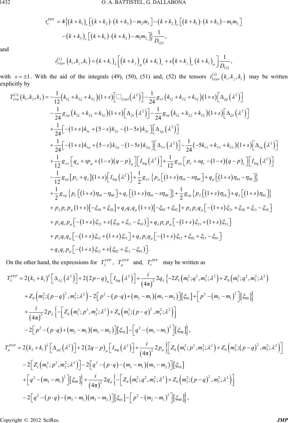



 

O. A. BATTISTEL, G. DALLABONA

1432



























1232321

31212

123

4

1,

PPV

tkkkkkkmm kkkk

kkkkkkmm D







 



 



313

kkmm



 

and



3,,

sijlij lj

tkkkkkkkkkskkk

 



  

123

1,

l

kD











with 1s . With the aid of the integrals (49), (50), (51) and, (5



,,

sijl

tkkk



may be written

explicitly by

2) the tensors 3



 



  

22

1231 231 23

22

123 123

2

123

132

11

,, 11

12 24

11

24

11515

24

11515

24

s

Tkkkkkk sgkkk s

gkkk sgkkk s

sk sksk

   

  

 

 





 



 

 



 













□



11

24





 



 







 





22

123

22

log log

2

log100001 00

10 00

151

24

11

12 12

11

111

12 2

11

2

kkks

gqsps qpIgpsqsqpI

gpqsI gpssqs

gp sq



  



 

 



























 











 













 















 

01 001001

30200302212011 10

212011 102111

12 11

1

111

2

11 1

111

11

ssgps qs

ppp sqqq sppqs

pqps sqppss

pqqss qpq

 

 

  

 

 

 

 



 



























1202 11 01

120211 01

1

1.

s

qqps s

 















On the other hand, the exVPP

T



pressions for ,

P

VP

T



P

PV

T



may be written as and,









 















22222 222

31log11 301 3

2

2 2

2222 2

0232132012100

2

222 22;,;;,

4π

;,;2

2

VPP i

TkkpqI qZmqmZmqm

Zmpqmppqmm mmpmm

i

ppqm



 







22 22222

01 2023

22;

,;;,;

4πpZ

mpmZmpqm



2 2

;







 

 

 



 















2

132 103100

,mmmq mm





 









 

























222222

21log01 202

2

22 222

1123 1 3210

22

222222

31 00013023

2

222 2;,;

4π

2;,;2

2;,;;,;

4π

2

PVP i

TkkqpI pZmpmZm

Zmpmqpqmmm m

i

qm mqZmqmZmpqm



 



 





2

222

3

22

;,;

pqm









 

 





 















 



 















2

22

31 3 2012 100,qpqmmmm pmm





  



O. A. BATTISTEL, G. DALLABONA 1433

























22 2222

32log01 202

2

2222

123312 1103 100

2

222222 2

0130231

2

22;

4π

2; ,;2

2;,; ;,;2

4π

PPV i

TkkpqIpZmpm Zmp

Zmpqmpqmm mmqmm

iqZmqm ZmpqmZ







 





2

222

3

,;;,;

qm











 

 





 





6.4. The Four-Vector Four-Point Function

four fermioni

ur-vector four-point function, given by

 



 



 





















2

222

23

2

3121 012100

;,;

2.

mpqm

pqmmm mpm m



















Finally, in the next section we perform the calculation of four-point functions.

As an example of calculation of a Green function of the perturbative calculations havingc propagators, we

consider the fo

11223 3

11 1

VVVV

tTr

kk mkkmkkm

 



 4 4

1

,

kk m











or





















3

12 4

123 4

12 3 4

1234

12

34

12 13

121 2

1234

2

1

23 1

14 23

121 2

1234

VVVV kk kkkkkk

tTr D

kk kkkk

mmTr mmTr

kk kkkk

m mTrmm Tr

D



 

 





12

24

1234

kk

DD







  



  

  

 

 

 





 













12

4

1234

12

1234

kk

D

kk

DD

2

1

13

24 34

12 12

1234

1.

kk kkkk

mm Trmm Tr

mmmmTr D







After performing the Dirac traces we identify the following structure

VVPP

gt

 

 

 

  









4

.

VVVVPPVVPVPVPVVP VPPV VPVP

PPPP

t tgt gt gt gtgt

gg gg ggt

 

 



















(73)

d usl tenstemced



;

1234

,,;,kkkk







(74)

where

In the above expression a convenient anefusorial syatization was introdu



;;;

;1234; 1234;1234;

;;

; 1234; 1234

,;,,;,,;

,;,,;,,

ttkkkk tkkkktkkkk t

tkkkk tkkkk

  

  

  

 































;

12

4; 1

2

,;,

ijlni ji

ln l

tkkkkkkkk kkk

kk kkkk



 

 



  



1234

1.

j

n

k

kk D

















(75)

1

Here and 2



assum the values 1. We also see that the coefficients of the metric tensor are four-point

amwith vector aneudoscalar vertices defined as

e

d psplitudes

12 3 4

123

11 22 33

111

tTr

kk mkkmkkm



   

 4

44

1

.

kkm









O. A. BATTISTEL, G. DALLABONA

1434

After performing the Dirac traces, the four-point amplitudes with vector and pseudoscalar vertices acquire the form



2

1 3

1 4

2

kk

k

 





 





 

 





 



12 3 4

13 4341221

32 424134

52 323146

71 414238

4

ts kkkkmmkkkkskk

s kkkkmmkkkkskk

skkkkmmkkkkskk

 







 









 











 















 















3

2 4

4

k

kk



 







 











91 313 2410

11121 234123

13

4

4,

PPPP

skkkkmmkkkkskk

skkkkmmkkkks kk

sg t



















 











 









(76)

i





where



5,





 and 1

i

s and



55 5

112233

111

PPPP

tTr

kkm kkmkkm

 

 5

4 4

1

.

kkm











Below we identify the values of i

s

according to the corresponding amplitude

7 8 912341234 5 6

1011 1213

s

sssss

ss

PVPV

PVVP

VPPV

VPVP

VVPP

 sss





ss





PPVV





 























 









 









 









 









Some algebraic effort is necessary in order to obtain an expression for the above amplitudes. This is a tedious task,

although easy, because the number of external momenta and Lorentz indexes involved produce very large mathematical

expressions. Consider first the t=2j=3 and =4l. From the results (53), (54), (56), (59)

and, (62) we get

ensor (74) for =1i, , k









  







12

;2 222

222

2

12

1111

22

111

222

1

41

ss g g

ggg

srsqJ

  

  















  





 



 



























221

1221

212 1

41

41 4

44,

qsrJspJ spJ

sqrsqr JrsqpJspJ

qsrpJspJqrsqrpJ spJ



 

  

4; 1 2

11

62

Tss g

 



 

 

 

□

log12

41 1

6gg ggggIss J

   





 







 





 

 

 

 

 

 

O. A. BATTISTEL, G. DALLABONA 1435

J

where J





,





,





and



are given by in Equations (55), (57), (60) and (63). Replacing the above result

(with appropri1

ate values for the symbols and 2) in Equation (74) gives







  



222 2

111 4

222

ggg ggggggI

  

 





 

  







2 222

log

4111

322 2

3

32 16

Tggg

JrJpJqrJqp

  

 





 



 



 



 

 

 

□



















8

888

4

JprpJ

rq qrJpq qpJrpprpq qpJ

pqr qrpqr qrpqrqrJ

p

 

   

  





r











 

88qr rqrp prJqrqrpqqp prrp J

  



 

 

 





































4

4.

qr qrpqr qrpqrqrJ

pqr qrpqr qrpqrqrJ

  

  



 









For the amplitudes listed in the table above we may write

 

 

  

 







 





1234 22

1log0123

678913 ,

PPPP

TsgIgFppFqqFrrFp

pqFqpF qrFrqFsgT

 

 



 



  











45

rFrpF

 



where



000

6 000

1

s









  



 

2

02 003 004005 004312

2

22

4178 00031910 000

2

1

11

Fs ss srqmms

rmms sqmms s

pm







  

 





 



2

22 2

4234 000325

1rpmm ssqpmm s









  

















 

    

 

 





2

11112 000

1,mss



















































1220 320 52002 511191291010

177 81210111112797 891010

111112 7 9 78 910011112 00

2

1

22242

2222

2222 1

2

Fss ssssssss

sssssssss ssssss

ssssssssss s

srqm

 



   





  

 

 





 









 



222

4322002100342

2

2 2

2

53262007418200

22

2 2

9311020010 100112112

112

2121

2112

ms ssrpmm

sqpmmssr mms

sq mmsssp mms



 

 







 

 

 



 



 









4 200

8 100

1

s













200 ,



































230242052073017 83 40111123

2

2222 22

22 2

Fss ssssssssss

ssssssssssrq mm





 

 

 



 











0

2

2 2

2

326 0207418 020

22

93110 020112112020

12

212 1

qpmmssrmms

sq mmssp mms





 







 



 





10

1s













 

11 34 1011127 11 78 101432020

22

3424020401

21

1srp mmss







8 010

12 010

11,

1

s

















 



5

2s









O. A. BATTISTEL, G. DALLABONA

1436

















































32024025029 5 01910 5601115

11 12560111911 1291001

2

22

1432 002342

2

53

2222 22

22

212

2

Fsss sssssss

ss ssssss ss

srqmmssrp mm

sqpm

 



  

 

 

 

 

 





 



 

 

2

26 0026 001

2

22

7418 00293110 002

2

112112 00212 001

11

2121

211,

ms s

srmm ssqmm s

sp mmss











 

 

 

 











01

2

4 002

1

s













 

10 001

1s





 





























 



2021195 109 120111 9 1112910 11 78 01

2

119109 0000143

2 22

222

sss ssssssssssss

sssrq mm

 

 

 



 

 





 

4115

1121012 001

22

3424 101

2 1

21

ssss

srp mms



 















 



2

5326101

2

22

7418 10100193110 101100

2

112112 101100

21

2121

21,

sqp mms

srmm ssqmm s

sp mms

 











 

 

 

 











22F s





  

 

100

001 000









































 



 

11 9791011 12011112910109100011 1200

2

222

1432 101001342

22

222

212

sssss ssssssssss

srqmmssrp mm







 

 

 

 









 



2

2 2

2

53261016 1007418

2

93110 10110 001100000

2

11211210112 100

1

212

21

21,

sqpmmsssr mms

sqm mss

sp mmss





 



   





 













5211502119 101019 105610





4 101

1018 001

1

s















22 22Fs ssssssss

 

  































63115201173 107 120111127 11 78

22 2222Fs sssssssssss

 



 

  



 



 

2

11 127017001112001432110

22

3424 1101

22

22 1

21

sssssssr qmms

srp mms

  





 

 















 



2

005326

2

2 2

7418 11010001000093110

2

11211211012 100

21

21 2

21,

sqpmms

srmm ssqmm s

sp mmss



















 











9 1010

2 010

sss

s















110

110 010

1













 































7311520117 8101783 410111271178

22 222Fssssssssss sssss



 





117 8017 80011001432110

22

34241104

22

22 1

21

sssssssrq mms

srp mmss

11 9 10

2

010

s s



 

 

















6 110

s











 





  













 



2

100532

2

7418 1108 010100000

2

9311011010 010

2

112112 110100

21

21,

sqpmm

srm mss

sqmmss

sp mms

















 











O. A. BATTISTEL, G. DALLABONA

1437













































 



841151111 5 1011 9 1011 340111 78 01

2

222

1432 0113424 0114

2

532

2222 22

212 1

21

Fs sssssssssss

srqmmssrpmmss

sqpmms

11 0000

001

2s



 



  

  

 

 















2

6 01101074180118

22

93110 011010112112 011010

21

212 1

srm mss

sqmmsspm ms

 

 



 

 

 



 



  





 

 





001

001000 ,





















































 



 

941151111 1230111 1270111 125610

2

11 129101011 1200001432011

22 2

34240110015

222 2 2

222 1

212

F ssssssssssss

sssssssr qmms

srp mmssqp

 

 



  

 



 

 















 





2

3 26

2

22

74180110019311001110 010

2

112112 01112 001010000

1

2121

21,

mm s

srmmssqm mss

sp mmss

 











 

 

 

 









0116 010

s























00

2

000

2

.

rp

p



 













2

222222

log024012

22

00 00

22

222

00

42;,;,

22

PPPP

TI ZmrpmZmqm

qrqrpqp rrq

pqp prqqrprq













 









 

 





 















Above, the following compact definitions were also

used



222

123

;, ;,,mqm



222

124

;, ;,,

nmnm mpmrm







222

134

;, ;,,mrm



222

234

;,;,,pmr pm











112 34 56

01112

1

1,

s ss

nmnm mp







nmnm mq



 

nmnm mq





and



11sss s

78

91

11

s

ss s



2125

11sssss



s s



 

 

69 10

1,s s





4 78

11 1,





312 3

s

sss sss





434 56 1112

1,



11

s

ssss

ss





11 12

1.



5 78910

11

s

sss

ss s 

is point, fulfilled

oposed systematization

mplitudes. However,

another important aspect involved in perturbative calcu-

lations can be also considered which, within the context

of our procedure, became very simple and transparent,

that is the verification of relations among the Green

functions and, consequently, of the associated Ward

identities. We perform such task in the next section.

7. Relations among Green Functions

In the preceding sections we have described in details a

procedure to handle the divergences typical of the per-

turbative calculations in QFT. The procedure is very

general since all the choices involved have been pre-

served; the internal momenta were taken as arbitrary so

that all possible choices can be made in the final results,

the choice of regularization is avoided since all the steps

performed are allowed in the context of all reasonable

regularization prescription and an arbitrary scale was

adopted in the separation of terms having different de-

grees of divergent and finite ones. We can ask ourselves

at this point about the consistency of the perrmed op-

erations as usual in such type of manipulations and cal-

culations. In order to verify this aspect we can make a

minimal test of consistency by verifying if the relations

among the calculated Green functions remain preserved

after the realized operations. The required consistency is

to verify such identities without assuming particular

fo

Our main purpose has been, at th

which is to show how the pr

works in the calculation of physical a

O. A. BATTISTEL, G. DALLABONA

1438

choices for the involved arbitrariness, which means that

the relations need to be satisfied in the presence of poten-

tially ambiguous and symmetry violating terms. Essen-

tially, what we want to know is if the performed opera-

tions have preserved the property of linearity of the inte-

gration which seems to be a trivial task but, given the

mathematical indefinitions involved, it is not. Only if the

operations realized until this point possess the desired

consistency we can give an additional step which is to

verify if the potentially ambiguous and symmetry violat-

ing terms can be eliminated in a consistent way. Let us

consider this aspect in detail now.

We start by considering the VV two-point function

whose calculation we have considered in detail in the Sec.

(VI). In order to state a relation with other calculated

amplitudes it is enough to note the identity bellow



 





21

11

21

11

kk kk m

kk mk

mm kk m































 

2 2

11

.

kk m

k m

kk m



































After taking the Dirac traces in both sides we can

identify that

 

2 1,

VS

mmt





(77)

The above relation means that it is expected that if we

integrate both sides in the loop momentum k the corre-

sponding relation among the loop amplitudes remain

valid, i.e.,

 

2 1.

VS

mmT





(78)

This means that by calculating all the involved ampli-

tudes in a separated way and after this contracting the VV

amplitude the reorganization of the terms must allow the

identification of the amplitudes in the specific combina-

tion of the right hand side. This type of identity is highly

ontrivial to be preserved in traditional regularization

r

 

2 1,

SS

mmT

(79)

which implies that







21 21

2111 22

21 1122

2

21

,,

.

VV

SS

kk kkT

kk TkmTkm

mmTkm Tkm

mmT













 









 







(80)

We can note from the above expressions that all am-

plitudes of the perturbative calculations are related

among them. In particular, the above considered relations

involve the amplitudes: VV, VS, SS, PP, V and, S.

For the calculated three-point function structures we

can verify the relations





31

21233 1

,, ,

VVV

VV VVSVV

kkT

Tkk TkkmmT





 





 





 

(81)



 



21

13232 1

,, ,

SVV

SV SVSSV

kkT

Tkk Tkk mmT



















(82)



 

32

12133 2

,,.

SSV

SS SSSSS

kkT

TkkTkk mmT















(83)

Now we can note that all the three, two and one-point

calculated functions are in fact related among them

through precise relations. In the above considered rela-

tions the following structures are involved: VVV, VVS,

VSS, VV, VS and, SS plus the ones which appear as sub-

structures: VPP, SPP, PP and S.

If we consider four-point functions, the same will oc-

cur. To evaluate the VVVV function all the above men-

tioned structures will appear as well as other four-point

structures. This is a very crucial point. We can start from

a finite amplitude and by successive contractions we can

relate such amplitude with the cubically divergent one-

point function. The challenge is then to evaluate all the

perturbative amplitudes within a certain prescription

maintaining all the relations among them preserved in a

simultaneous way. Within the context of our procedure

we will show that all the relations presented above can be

verified in the presence of all remaining arbitrariness. We

emphasize that such type of verifications are very non-

trivial for all traditional techniques.

Let us start by the property (78). Taking the expression

for the VV amplitude, Equation (, and contracting

with 21

kkp





21

112 2

,,

VV

kkt

tkmtkm















21

112 2

,,

VV

kkT

Tkm Tkm











n

pescriptions. A similar procedure allows us to state that



 

21

112 2

,,

VS

SS

kkT

TkmTkm





 69)

 we get



O. A. BATTISTEL, G. DALLABONA 1439









12

21 21

211

22

101

12

,

2

4;

,.

VV

pTk k

mm mm

mmpZm

mpZmpm

pAkk











  













2

log

22 22

1 2

22

2

,;

pI

pm

















By comparing to the resu) for the VS mplitude

we can identify



2









lt (67 a





12 12

22

,,

2

VV

pTk kpAk k

mmkk



 





 



21

21 12

,.

VS

mmT kk













In order to complete the verification of the property

(78), the last term in the above equation must be identi-

fied with the one-point vector functions. It is simple to

note that if an





 is added and subtracted in the ex-

pression for

A





, a reorganization allows us to identify

 

VV

pAT kT k











.







22 2

2121

2mmk k









 



12

  



So, the relation (78) is obtained preserved by our

calculation.

The relation (80) is, on the other hand, emblematic to

explain many aspects of our procedure and we will make

the discussion in details. First we note that by contracting

the expression (67) for the VS amplitude it is obtained





2

12 1122

22

21 log

22222

12112

22222

101 2

2

4;,;

4;,;.

VS

pT

mm k kkk

mmpI

mmpZmpm

mpZmp m

















 



 





(84)

We know that this result needs to be related to the SS

amplitude as well as with S amplitudes having different

masses. This means that quadratic divergences need to

appear from the right hand side in a non-cancelling way.

At first sight it seems that it is not possible to satisfy the

relation. However, we note that on the left hand side of

the identity (84) we have the function Z1 and in the right

hand side only Z0 must appear. Let us consider the reduc-

tion of Z1 to Z0 through the property (13) in order to

adequate the right hand side of the Equation (84). The

referred reduction is the property (13) which allows us to

write





 

22222

11 2

2;,;pZ mpm



2222222

1201 2

22

22 22

12

11 22

22

;,;

lnln .

pmmZmpm

mm

mm mm















 

 

 

 

(85)

Now consider the result obtained for the 1

I

integral

at the value 0,

i

k



which is nothing more than a scale

property of the basic quadratic divergent object





2

quad

I,

















22222

quad 1quad1log

2

22 2

11

22

1

ln .

4π

ImIm I

imm

m



































(86)

We get then



 



2

22221

quad 1ln m

i

ImImmI











quad21log22

2

22 2

2log22

22

4π

ln

4π

m

i

mI































 

the scale properties of the divergent objects

22 22

12

11 22

222

ln ln .

4π

mm

immmm





 



 



 



Now note that we can relate the reduction of the finite

functions to





 

 



22222

11 2

222 2222

1201 2

22

2;,;

;,;

pZmpm

pmmZmpm

















quad 1quad 2

2

22 1

1log 22

2

22 2

2log 22

ln

4π

ln ,

4π

Im Im

m

i

mI

m

i

mI





Substituting in the expression for VS amplitude we

will identify the relation (79) among the Green f

VS, SS, and, S. Note that the precise connection

the finite functions and the basic divergent object allows

exact way the considered relation

ions. It is not necessary to emphasize

that the same procedure is nontrivial within the context

of traditional regularization methods.

Let us now consider the relations among the three-

point functions calculated in the previous sect

tracting the VVV amplitude, calculated in

with q







































unctions

between

us to verify in an

among Green funct

ion. Con-

last section,



and using the properties (23), (24), (25) and

(29) in order to eliminate the nm



functions having

3nm in favor of those having 2nm we get



O. A. BATTISTEL, G. DALLABONA

1440























 



log

222222

212 112

2

222

1121 2101

4

2;,;,

π

;,

I

igp ZmpmZmpm

mpmmmmZm







2

22

log

4

3

g pqpq pqI









22

21

4

mmZ

2

12 23

2

222

1223 log

4

,,

3

2

VVV

qTA kkA kkgppp

gm mmmI



 























 

 

 







 



































2

22222

332123

222

22 3

2222

02 3

;,

8 ;,;

; ;2

m mZm pq m

ppZmpqm

Zm pqq







 







 











22 22

2

22 2

22

223 1

22

222

23202 32

22

22222

12321

;,;

2;, ,

;,;

4π

2; ,;;,,

pm

pqZm pq mZmq m

i

mmmZm pq m

Zm pq mZmpm











 













 



2

;p





22

2

;m2

1120 10

pq q





 









 



22

22222

22 312 30211

2

3 101002

1

8;,; ;,;

2

4π

11

22

4π

iqqZm pqmZm pq mqpq

qmm p



















22

22

2222

22 3123

;

,;;,;Zmpqm Zmpqm

 

8

iq







 



 













2

22 2222

01 2023

1;,;;,;

4ZmpmZm pq m



















  





 









2

3 01

2

222

23123

2

;,;

m

mp qm





















2

22 2222

01 2023

1;,;;,;

4ZmpmZm pqm













2

2222

1230211

22

1 0000

1;,;

2

1

2

Zm pq mqpq

m q



















 



2

31 2 110

2

222

2

11

24

8;

,;

4π

pqmm mmq

ipqZmpqmZ



















  





















 













 











22

11 20 0110

2

003 1003 1

130013

2

1

2

11

24

48

4π

qp

q qpqq

qmm mm

igmmmmp

 





















 







 











13 11 1311

88

p

mm

qp mmpq

 



 

Given the obtained result, we now use the properties (1

22 222

11 20211

2

3 1312 110

22

1

1;,;

2

Zmpmqpq

pqmmmmmm

mm gI

 



















 





 



g







9) a

3 log

 











201 302

8

.

SPP

mmqq

T











nd (20) to eliminate the nm



functions having 2nm





in favor of those having 1nm. We get then













2

2 2

log log

2222222

4

3

2;,;,

g pqpq pqI

gp ZmpmZmpm

 







 



2

22

12 23log21211 2

2

22 222

2111221101

24

4π

;,

I

i

gm mmmI

mmZmpm mmmZm





2

12 23

4

,,

3

VVV

qTA kkA kkgppp

 



















 





 

 





 





 











22 22

2

22 2

2222

22323

22

2222 222

321233 22023

2

2222

22312

2

;,;

2;,;,

;,;,;

8;,;;

4π

pm

pqZm pqmZmpqm

mmZmpqm mmmZmpqm

ippZmp qmZ m













 





 

 

 

 









1





2

22

3

,;pqm



O. A. BATTISTEL, G. DALLABONA 1441





 





 







22 2222 2

21 211

;,; ;,;Zmpm Zmpm







2

22

222222

223123

2

22

222222

223123

2

22 222222

0 120230110

8;

,;;,;

4π

8;,;;,;

4π

1

;,;;,;

42

iqqZmpqmZm pq m

iqpZm pq mZm pq m

ZmpmZm pqmqpq







































1







 

















 



2

31 00

22

222222

22 3123

2

22 2222

0 12023

22

31 13log

1

4

8;,;;,;

4π

1

;,;;,;

4

24

qmm

ipqZm pq mZmpqm

ZmpmZm pqm

mmmmgI



 









 























 



 





02

1 311012 110

42pq m mmmg

 



 

2

2 2

01103 100

2

1

24

4π

qpqqm m

ig























 













1300

1 011311012110

42

mm

mqp mmmm





 



2



1320 1013

88p

pmmqq mm

 





.

SPP

T





 





 











Finally, using relation (17) we write







 



 













222

12 log

222222 2

21 211 221112

2

22 222

2110121223 log

4

23

8;,, ,

4π

4;,;,2

4

3

VVV

qTgmmIgpp pI

igpppZmpmZmmm

gmmmZmpmAkkgmmI

gp



 

 

 







 

 

 



 



 



 



 







2

log

2222

4;

gm mZmp











2

;

p

 









  

 

22

log

222

2222

22 312 3

2

22

22 22222

321233 22023

22

233 11 3log

8;,;,

4π

4;,4 ;,;

,2

qpqpqI

igpqpqpqZmpqm Zmpqm

gmmZmpqm gmmmZmpqm

AkkmmmmgI



 

 







 





 



















 











 

 



 





1 3001320101 302 101

2

13110121101 00

1 311012 110 100

488

4π

42

42 ,

SPP

igmmppmmqqmm m

qpmmmmm

pqmmmmmg T

 



 



 







 





 









If we consider the results for thplitudes VV and

SVV , Equations (69) and (71) to note that

the expression above may be id as being the

relation (81). It is not difficult to verify the relations (82)

and (83) by performing the same sequence of steps.

The procedure used above can also be adopted to state

analogous constraints to the four-point Green function.

As an example of such constraint we have



 



41

123 234

41

,, ,,

.

VVVV

VVV VVV

SVVV

kkT

TkkkTkkk

mmT



 

 







e am

, it is now easy

dentifie



 





 







In order to show that the calculated four-point ampli-

tude VVVV satisfies this relation, at first we contract Eq-

uation (73) with



41

kk



 and eliminate the ijk



O. A. BATTISTEL, G. DALLABONA

1442

having i + j + k = 1 in favor of those having i + j + k = 0.

The next step is to use the properties (34)-(43) in order to

eliminate the ijk



and ijk



functions having i + j + k =

favohose having i + j + k = 3 and so on. The

latioeasy but involves a lot of algebra, therefore

we will now it explicitly. All the required ingredi-

have given in the preceding sections.

8. Ambiguities and Symmetry relations

e Sect6 we have evaluated, within the systema-

on ped, Green’s functions which are typical of

erturb tive calculations. In particular, all the con-

d amudes appear in the context of Standard

. the evaluated Green’s functions, having

ee ofrgences higher than the logarithmic one, it

is possible tnote the presence of terms where the de-

nce he internal momenta appear as arbitrary

tities (th summations of them). This is expected

ce a sh in the integrating momentum generates sur-

faces terms which implies that different choices for the

ernal lines momenta lead to different am-

udes.possible dependence on the choices for the

ls of tnternal lines momenta characterizes what

enoe as ambiguities. This situation is not ac-

in this case, the power of predict-

of thry is destroyed. In addition, fundamental

tries like the space-time homogeneity

are not prese ved in the perturbative calculations. It will

sung to find global and local gauge symme-

tries as well as internal symmetries violated in physical

itudes ving the space-time homogeneity broken.

ere is onone possibility to save such type of calcula-

oinate the ambiguous terms in a consistent

niv way. Within the context of the adopted

gy tbiguous terms are automatically separated

d preservso that it is easy to identify them.

one-point function it is simple to identify



2

1

4,kk













4 in

calcu

ents

In th

tizati

the p

sidere

Model

degr

pende

quan

sin

label of t

plit

labe

we d

tion

space-tim

not be

ampl

Th

tions: t

and u

strate

an

In th

r of t

n is

t sho

been

ion

ropos

a

plit

In all

dive

o

on t

e

ift

he int

This

he i

minat

ceptable just because,

e theo

e symme

r

rprisi

ha

ly

elim

ersal

he am

ed

e case of

ambiguous 11

S

Tm

















22 2 2

111

2

111

2

111

22

2

4

3

2.

kmk

kkk































 













□

In the tnt functions we get

2

1

ambiguous4

V

Tk





 

 

wo-poi





2,P













2

2,

SV mP















2

ambiguous,

PP

TPP





ambiguous





  

 





 



22

ambiguous

2

22

2

1

2

13

3

13.

6

VV

TP

PP pP pP

PP PP

gPPpPpP

 

 





 

 

 









 

 









 









□

In the case of three-point functions we found



2

31

ambiguous2,

VSS

Tkk









  

 



2

31

ambiguous 2,

VPP

Tkk









 

 



2

21

ambiguous2,

PVP

Tkk









 

 



2

32

ambiguous 2,

PPV

Tkk









  

 



2

123

amb

2

231

2

123

2

132

2

123

2

123

2

123

4

3

222

3

222

3

222

3

222

3

222

3

222 .

3

VVV

Tkkk

gkkk

kkk







 



 



 

















 

 



























 





 



□

In all the above listed ambiguous terms it can be noted

that they invariably appear as multiplying the objects ,





and, □. All these terms present simultaneously

scale ambiguities because such objects are dependent on



. This is due to the fa

SS

TP









21

Tm

  



the arbitrary mass scale ct that in

all amplitudes the obtained expression is independent of

the parameter 2 if the terms containing the objects ,







and, □ are absent. This statement can be verified

directly by differentiating the expression or changing the

scale to another one, like for example one of the involved

fermionic masses, through the scale properties of the

finite function and of the basic divergent objects





2

quad

I





2

log

I and . The referred properties are









 



22222

quad 1quad1log

2

22 2

11

22

1

ln ,

4π

ImIm I

imm

m



































O. A. BATTISTEL, G. DALLABONA 1443

,

 



2

1

22

ln ,

π

m

i











22

log 1log4

Im I





22 2222 22

121

2

1

2

;,;

,

pm



















12

2

;,;

1ln

1

kk

Zmpm Zm

k









2222 2222

1232 1231

2

1

2

;,;,;;,;,;

ln .

11

nm nm

mpm qmmpmqm

1

nm

















xpressions for

the perturbative amplitudes which are nonambiguous

relative to the choice for the internal lines momenta, but

are ambiguous relative to the choice for the common

scale for the finite and divergent parts. This aspect can be

easily noted in the considered amplitudes. In the VV

two-point function

 



This means that there are terms in the e



 



scale_amb

222

12

22

2

422

55

66

11

33

1.

3

mm

pg

pp pp

pp





 



 











  





 













□

In the SVV amplitude

22

2

22

VV

T

pp



































2

13

2,

SVV

Tmm

 





 

 

scale_amb

and in the VVVV amplitude

 



scale_amb

2

42

33

44

33

24

33

4.

3

g

gg

g

 

 

 

 

















 









□

In such examples the listed term

22

VVVV

T





 

 

























s are independent of

the choices for the internal momenta. They can be con-

verted in ambiguities through their evaluation in inter-

mediary steps within the context of traditional regulari-

zation techniques. Again we can note that all the poten-

tially scale ambiguous terms are combinations of the

objects





and, □.

Let us now consider the symmetry relations. It is easy

to see that the situation is completely similar to the ques-

tion of ambiguities considered above. There are two

types of impositions coming from the symmetries for the

amplitudes. The general ones, coming from Lorentz and

CPT, present in the Furry’s theorem, whose implication

states that all amplitude which has an odd number of

external vectors and only one species of fermion at the

internal lines must vanish identically, and that coming

from the divergence of the fermionic vector current

which states a precise relation with the corresponding

scalar current. The first of the impositions mentioned

above implies that the amplitude



1

V

Tk



must be iden-

tically zero, which means that it is required



s















2

1

22 22

111

2

111

2

111

04

222

4

3

2.

k

kmk

kkk

























 





 













□

Due to the same reasons, the theorem states that the

amplitude for the process VVV, which is the VVV

amplitude symmetrized in the final state,





123 123

,,,, ,

V VVVVVVVV

TTkkkTlll

 



must vanish for the case of equal masses. The arbitrary

internal momenta for the second channel obey, 21

qll





and 31

pl l. This means that it is required







2

123

2

231

2

123

2

132

2

123

2

12 3

2

123

4

03

222

3

222

3

222

3

222

3

222

3

222

3

,.

ii

kkk

gkkk

kkk

kl







 



 



 



















 



























 





 



 

□

Concerning the symmetry relations coming from the

proportionality of the divergence of the fermionic vector

current with the scalar current, we note that in the VV

two-point function we get

O. A. BATTISTEL, G. DALLABONA

1444



  







2

log

22 22

1 2

22

2

,;

pI

pm

















By comparing to the resu) for the VS amplitude

we can identify





2

1

2

,,

k

















which means that the symmetry relation is broken by the

terms which are all combination jects





12 2 12 1

21 1

22

101

12

,2

4;

,.

VV

pT kkmmmm

mmpZm

mpZmpm

pAkk











 









lt (67







12 12

22

212

21 1

,,

2

VV

VS

pTk kpAk k

mmkk

mmT k



 







 



of the ob



,



and, □. In fact this result require as the Fur-

ry’s theorem, a vanishing value fotor one point

function. Following this line of reasoning we note that

the SVV amplitude possesses a symmetry violating term

which is independent of the choice for the internal lines

menta

es the sam

r the vec

om







13

sym_break 2.

SVV

pTmmp q



 





 



The same occurs for the VV VV process where

the violating term is proporcional to



2



2







□ with a

nonanbiguous coefficient.

In view of the above comments and others omitted, it

is very simple to conclude that all these unwanted prob-

lems can be removed from the amplitudes in a consistent

way. There are simple but powerful arguments. If we

consider that a perturbative solution for the amplitudes of

a QFT must be compatible with the space-time homoge-

neity or it does not make any sense, if we cannot admit

that the scale independence can be broken by any method

or

tion

nm gra

that

we denominated them as Consistency Relations. Such

conditions can be easily understood. In fact the definition

of the objects ,





and, □ has been conveniently

made in order to get clean and sound clarifications. First

note that





2

2222 22

2,

kgkk

kkk

k

























(87)



223

222222

4,

kgkk

kkkk





















(88)

 



333

2222 22

34

22 22

6,

kkkkk kk

gg

kkkk

kk kkkk

gkk

 

 



 

























(89)

so that we can identify



strategy adopted to give some meaning for the pertur-

bative amplitudes and if we also cannot admit that an

acceptable interpretation for the perturbative solu

breaks symmetry relations of the underlying theory, then

it becomes necessary to impose a set of properties for the

divergent Feyan intels in order to recover these

symmetries, due to the fact that the perturbative series is

not automatically translational and scale invariant and

symmetry preserving. Fortunately all these problems can

be solved simultaneously. It is enough to impose

0. □

We can look at these conditions as a set of properties

required to a regularization method in order to produce

consistent results or we can think that this is the set of

properties required to the perturbative series in order to

get the space-time homogeneity maintained in the calcu-

lated expressions (among others). Due to these reasons



4

422

d,

2π

k

kk





















 (90)



4

42

22

d,

2π

k

kk





















 (91)



4

43

22

d1

.

4

2π

kkk

k

kk

























□ (92)

The factor 4 in the last condition is justified by the

symmetrization in the Lorentz indexes. In order to give

symmetrical role to all indexes four terms need to be

introduced in the left hand side given the factor 24 to the

fourlinear in loop momentum integral. Frequently it is

convenient to write such integral in symmetrized form.

We adopted the definition of the object □ in a non-

simmetrized way only to reduce the mathematical ex-

pressions. Note that through the Gauss theorem these

quantities are identified as surfaces terms. It becomes

clear now that if these conditions are not imposed the

perturbative calculations simply does not make any sense.

It is on the other hand simple to verify that these condi-

tions are satisfied in the presence of any distribution.

W

and gauge symmetries are violated as well as the ampli-

tudes may be ambiguous quantities. Tprescription is

universal since in other dimensions as well as in theories

or models where higher degree of divergences are pre-

sent analogous conditions can be identified. This inter-

pretation of the perturbative calculations provides us the

required consistency. The calculated amplitudes are am-

biguities free and symmetry preserving.

ithout these conditions being fulfilled space-time, local

he

O. A. BATTISTEL, G. DALLABONA

1445

If one agrees with the arguments put above then the

adoption of a regularization become completely unnec-

essary for any purposes in the perturbative calculations.

All the required manipulations and calculations, inclu-

ing the renormalization, can be performed, following or

strategy, without any mention to the word regularization.

And, which is better, the results are so consistent as de-

sirable and no restrictions of applicability exist.

9. Generalizations of the Finite Functions

and Their Relationship

Through the proposed method to manipulate and calcu-

late divergent integrals, in the above sectionwe have

been learning how to systematize the finite parts of the

one, two, three, and four-point integrwhich are pre-

sent in the relevant amplitudes belonging to fundamental

theories. It is not hard to see that this systematization

could be generalized to amplitudes with an arbitrary

number of points. In this section we discuss some aspects

of this generalization. We begin by defining theet of

functions

where 1,2, 3,k



, and



1

1,

n

l

nl









with



being the Euler-Mascheroni constant. The fol-

lowing shorthand notation has also been used

11

1111

112

0000 1

ddddd,with ,

k

x

kki

i

x

xxx xx















d

u





,;; ,,QQmxpmx

 



11 211

,1

22 2

11 1

1

;,

.

kk k

k

ijiij j

ij

k

ii

i

mp

ppx x

mmxm











 





with

s

als

s







1

2

,,1121

1

;,;; ,;

ddln1 ,

if 0,1,2,

k

n

iik k

n

i

mpm pm

QQ

xxxx n

n



11 2

0!

kk

n



































(93)

1,, 3,



(94)







1

,,1 121

1

11

0

;,;; ,

dd if

k

n

iik k

n

i

kk

mpm pm

xxxxQ n











 2



representing a Kronecker delta symbl. All fi-

nite parts of the one-loop Feynman integrals with an ar-

bitrary number of points, handled by the proposed ap-

proach, can be systematized through this set of functions.

We recognize that Equation (93) is the generalization of

definitions (12), (16) and (33) and Equation (94s the

generalization of Equations (15), (32) and (31).

In the preceding sections we have systematically eva-

luated the one, two, three, and four-point vector ampli-

tudes and verified their Ward identities. Within our ap-

proach, the verification of the Ward identities is greatly

simplified by using a set of identities characteris-

tic



n





o

) i

of 1,,

k

ii



, like those given by Equations (17)-(29). In

order to obtain such identities for an arbitrary number of

points first we note that











12 123

12

2

11,,,12, 1,,,1

222

1112

112 ,,,

2

01

1ddln 1,

2! 2

kk

k

nn

iiiiii i

n

i

ii

kk iii

ppp p

mm

Q

QQ

xxxxxn

xn



 





  

 

  









 



 















where 0n and 12

,, ,0,1,2,

k

ii i

12 11

,,, ,

kk

n

kii ii

p





 

 





. After an integration by parts, the first term on the right hand side of the above

equation may be rewritten as

   

1

11

111

2 2

0

ddlnddln2 .

1! 1!

k k

n n

i i

kk kk

QQ QQ

xxxxnixxx xn

xn n

1

11

02



1





 















 











e in 1



x

The first term is a total derivativ. So, performing the integral over 1

x

, we write the above expression as







  



 



 

1

12323

11

22

21

,1 ,022

1

22

211

2

,0,1, ,,, ,,1

ln 2ln 2

1!

21

kk

nn

ki

n

nn

i kiiiiii

mm

nn

mm

 



 













 





  

 



 

  





 

 

 







123231

12 1

1

,,,

00 0

,

k

llillil

ll l







 







1! 

1

,1 ,0 2

,

1l

n

1!

1

ki

k

ni

n



















2

11

1

1112

1,

0

1

k

l

il n

i

illi













 





O. A. BATTISTEL, G. DALLABONA

1446

where



2

1

; ,;,

kk

pm





2

212 311

;,;;,;,

kk

mp pmp pm







  







11 2

;, ;mpm









2

1

;,;,

kk

pm



223

;,;mpm









1

11

1

...

11 12211

1! .

!! !!

k

l

i

ll kkk

i

il lllll





 





Finally, we get a recurrence relation



1123 12

2

1

111212323112323

1

,1,,,1 ,,,1

11

,, ,,0,1,, ,,, ,

00 0

1

kk k

k

kkk kk

k

nn n

iiiikiii

lnnn

i

llillill ilikii iii i

l

p pp











 







 



 



 

 





 

 







2

11,, 12

ii

il

pp









11

12

,1 ,0

11

kill





 



 



 



 



1

2

1

2

22

1

2

222

112, ,

ln 2

1!

1.

2k

n

ii

m

2

,1 ,0 2

1

22

,1 ,02

ln 2

1!

1ln2

1!

n

ki

n

ki

m

mm

n

pmm

 



 



n

mmn

n





 













 







 



 







 

 













is





























 









Extending these relations for functions with arbitrary n



straightforward. The result is very similar









3 2 3112323

,1 1

,...,,0, ,,,

k

k k

k

kn

illiliiiiii

p







 





 

 







1123

11

112 1 2

12

2

11,, 12,1,,,1

2

,0 1

,1... ,

00 0

1

kk

k

nn

ii iiii

l

il k

in

i

kllill

lll

k

ppp p















 



  

 

  





 

 









12

,,,1

1

k

n

iii







 

 







 



 



1

,,

1

2



 

1

2

1

112 ,,

,

2k

ii

p

mm

22

1

2

222

ln 2

1!

1

k

ni

n

m

2

,0 2

,1 2

1

22

,0 22

,1 2

ln 2

1!

1ln 2

1!

n

i

k

n

i

k

m

mm

n









n

mmn

n























 







 

 

 







 

 













(9

1if 1

nn

n











The symmetry of



1,,

k

n

ii



 functions by interchanging

momenta and masses



1,, 11

2

,

k

n

iij jj

n

ppmm

mpm pm













 

 







 



















with





5)



111 2 1

;, ;; ,;

where 2,3,4

jkk

ii

j













may be used to get more 1k similar identities. If we

perform this operation in Equation (95) we get a system

of linear equations given by



12

1, ,,

11 1211

k

n

ii i

k

pp ppppb







 

















12 3

12 1

21 22 22

,1,,,

12 , ,...,,1

,

k

kk

n

kii ii

n

kk kkk

iii i

pp pp ppb

pp ppppb









 













 















with













 

12 1

1

00 0

1

22

2

,0 2

2

ln 2

1!

k

ll l

n

immn

n







 





















2

11

112 1 232 3112323

,0 ,1

111

1,1,. ,0,,,,,,

,1

1

k

kkk kk

l

il

ik

nnn

i

kllilllliliiiiiii

k

b





 











 

 















  





,

i



1



 



 











1

12

222

2

112 ,,

2

1

ln 2,

1!2 k

n

ii

pmm

 





1

,0

,1

1

2 2

2,0

1 2

1

,1

2

1

ln 2

1!

k

n n

i

k

mm

nn



























 

1

22

2

ln 2

1!

n

mmn

n









 

 





 



i









































O. A. BATTISTEL, G. DALLABONA 1447

with the j-esimo term given by



111

;

jjjj

bbp pmm



  and 1

j

ii. If, in a par-

ticular kinematical situation, the matrix

A

11 121

21 222

12

,

k

kk kk

pp pppp

 





 







 









A

has det0A, the solution of the above system of linear

equations can be written in a formal way by



12

1, ,,1

1

1,

det

1,

k

n

ii ijj

j

k

n

b









A

12 3

,1

,,, 2

1

det

k

ii iijj

j



A

r e

number of mathematical structures saving, in

this way, considerable computational time.

10. Conclusions

In the present work we considered general aspects in-

volved in the calculations of perturbative ampli

QFT’s. A very general procedure is presented for this

purpose. The work can be considered as an extension of a

previous one where only one species of fermion has been

considered [2]. In addition, the calculations in the present

contribution have been done by adopting an arb

scale parameter putting the calculations in the most gen-

eral way. All the arbitrariness involved in the calcula-

tions were preserved in intermediary steps. The adoption

oided, the internal momenta are

assumed as arbitrary and the common scale for the finite

and divergent parts was taken as arbitrary t

integrals were not really evaluated. Only

properties of such quantities were used. This became

possible through a convenient interpretation of the

Feynman rules. The perturbative amplitudes

for one value of the loop (unrestricted) momentum are

not integrated before a convenient representation for the

propagators is assumed. When the integration is taken all

the dependence on the internal arbitrary momen

sent in finite integrals. In the divergent ones no physical

quantity is present. Only the arbitrary scale appears there.

Th

t

11

,,

1,,

1

1,

det

ll l

k

nii i ljj

j

b















A

where ij

 is the cofactor of iji j

app. By recursive

use of the above relation it is possible to reduce all

functions



1,,

k

n

ii



 to functions with 12 0

k

ii i .

This type of reduction is useful, for example, in

applications whe e w are interested in numerical results

because within this procedure we have to manipulate

only a low

tudes of

itrary

of a regularization was av

oo. Divergent

very general

after written

ta is pre-

e divergent parts are written as a combination of stan-

dard mathematical objects which are never really inte-

grated and the finite parts are written, after the integra-

tion is performed, in terms of finite structure functions.

So, two very general types of systematization are pro-

posed;

1) Divergent parts. The divergent contenof one loop

amplitudes perturbative amplitudes belonging to funda-

mental theories can be written as a combination of five

objects;





2

log

I



,





2

quad

I



,



2





□,





2







and





2





.

2) Finite parts. The finite content can be written as a

combination of only three functions





22

0;

Z

pm ,





00 ,pq



and





000 ,,pqr



for amplitudes having two,

three and four internal propagators.

All self energies, decays and elastic scattering of two

fields can be calculated by using the results presented

here as well as their symmetry relations can be verified.

The results written in terms of the systematization above

can be used in the context of regularizations since all the

operations performed are valid in the presence of any

reasonable regularization distribution. All we need to

evaluate is the standard divergent objects.

As a last comment we argue that if we want to give

some meaning to the perturbative calculations we have to

impose that the space-time homogeneity and the scale

independence need to be recovered. Otherwise, the am-

plitudes become completely arbitrary quantities as well

as local and gauge symmetries may be violated (invaria-

bly by the ambiguous terms). If we agree with this argu-

is

□,

ment, our procedure makes this job easy. All we need

to impose that the conveniently defined objects







and







become identically vanishing. This as-

sumption can be viewed as completely reasonable since

these objects can be identified as surfaces terms which

are really vanishing quantities in the presence of any dis-

tribution. The same will occur by assuming the analytic

continuation of the integrals to a continuum and complex

dimension which is the ingredient of the dimensional

regularization. So, in any consistent interpretation of the

perturbative amplitudes only the basic divergences





2

log

I



and





2

quad

I



will remain in a calculated

divergent amplitude. They need not to be calculated since

they will be absorbed in the renormalization of physical

parameters. The calculation of beta functions can be done

by using the scale properties of such objects.

All these comments allow us to conclude that within

the context of our strategy the amplitudes are automati-

cally ambiguities free and symmetry preserving and no

regularization method needs to be used for any purp

The strategy, in addition, is universal since it can be ap-

plied to any theory or model, renormalizable or not, and

formulated in odd and even space-time dimensions in an

ose.

O. A. BATTISTEL, G. DALLABONA

1448

absolutely identical way. And, which is still better, the

results are as consistent as desirable. Investigatio

volving higher space-time dimensions (odd and even) as

well as nonrenormalizable theories in four dimensions

are presently under way and the obtained results are in

accordance with our best expectations.

In addition, other authors have been made investiga-

tions by using the procedure adopted in the present work.

In particular in [31] the authors explored some very in-

teresting aspects of the systematization proposed in [2]

concluding that there are important advantages relative to

the traditional ones.

REFERENCES

[1] O. A. Battistel and G. Dallabona, “Scale Ambiguities in

Perturbative Calculations and the Value for the Radia-

tively Induced Chern-Simons Term in Extended QED,”

Physical Review D, Vol. 72, No. 4, 2005, Article ID:

045009.

[2] O. A. Battistel and G. Dallabona, “A Systematization for

One-Loop 4D Feynman Integrals,” The European Physi-

cal Journal C, Vol. 45, No. 3, 2006, pp. 721-743.

doi:10.1140/epjc/s2005-02437-0

ns in-

[3] G. Passarino and M. Veltman, “One Loop Corrections for

e+e− Annihilation into µ+µ− in the Weinberg Model,” Nu-

clear Physics B, Vol. 160, No. 1, 1979, pp. 151-207.

doi:10.1016/0550-3213(79)90234-7

[4] W. L. van Neerven and J. A. Vermaseren, “Large Loop

Integrals,” Physics Letters B, Vol. 137, No. 3-4, 1984, pp.

241-244.

[5] G. J. Oldenborgh and J. A. Vermaseren, “New Algo-

rithms for One Loop Integrals,” Zeitschrift für Physik C

Particles and Fields, Vol. 46, No. 3, 1990, pp. 425-437.

[6] A. I. Davydychev, “A Simple Formula for Reducing

Feynman Diagrams to Scalar Integrals,” Physics Letters B,

Vol. 263, No. 1, 1991, pp. 107-111.

[7] Z. Bern, L. J. Dixon and D. A. Kosower, “Dimensionally

Regulated One Loop Integrals,” Physics Letters B, Vol.

93, pp. 299-308.

between Feynman Integrals

e Space-Time Dimension,”

Physical Review D, Vol. 54, No. 10, 1996, pp. 6479-

6490.

[9] R. G. Stuart, “Algebraic Reduction of One Loop Feyn-

C

doi:10.1016/0010-4655(88)90202-0

302, No. 2-3, 19

[8] O. V. Tasarov, “Connection

Having Different Values of th

man Diagrams to Scalar Integrals,” omputer Physics

Communications, Vol. 48, No. 3, 1988, pp. 367-389.

[10] J. Campbell, E. Glover and D. Miller, “One Loop Tensor

Integrals in Dimensional Regularization,” Nuclear Phy-

sics B, Vol. 498, No. 1-2, 1997, pp. 397-442.

doi:10.1016/S0550-3213(97)00268-X

[11] G. Devaraj and R. G. Stuart, “Reduction of One Loop

Tensor Form-Factors to Scalar Integrals: A General

Scheme,” Nuclear Physics B, Vol. 519, No. 1-2, 1998, pp.

483-513. doi:10.1016/S0550-3213(98)00035-2

[12] J. Fleischer, F. Jegerlehner and O. V. Tasarov, “Algebraic

duction of O Feynman Graph Amplitudes,”

Nuclear Physi c s B, Vol. 566, No. 1-2, 2000, pp. 423-440.

doi:10.1016/S0550-3213(99)00678-1

Rene Loop

[13] G.’t Hooft and M. Veltman, “Scalar One Loop Integrals,”

Nuclear Physi c s B

o

, Vol. 153, 1979, pp. 365-401.

d i:10.1016/0550-3213(79)90605-9

[14] T. Binoth, J. P. Guillet and G. Heinrich, “Reduction For-

malism for Dimensionally Regulated One-Loop N-Point

Integrals,” Nuclear Physics B, Vol. 572, No. 1-2, 2000,

pp. 361-386. doi:10.1016/S0550-3213(00)00040-7

[15] T. Binoth, J. P. Guillet, G. Heinrich and C. Schubert,

“Calculation of One Loop Hexagon Amplitudes in the

Yukawa Model,” Nuclear Physics B, Vol. 615, No. 1-3,

2001, pp. 385-401. doi:10.1016/S0550-3213(01)00436-9

[16] A. Denner and S. Dittmaier, “Reduction of One Loop

Tensor Five Point Integrals,” Nuclear Physics B, Vol. 658,

No. 1-2, 2003, pp. 175-202.

oid :10.1016/S0550-3213(03)00184-6

[17] G. Duplancic and B. Nizic, “Reduction Method for Di-

mensionally Regulated One Loop N Point Feynman Inte-

grals,” European Physical Journal, Vol. 35, 2004, pp.

105-118.

[18] G. Duplancic and B. Nizic, “Dimensionally Regulated

One Loop Box Scalar Integrals with Massless Internal

Lines,” European Physical Journal, Vol. 20, 2001, pp.

lus o

Integrals,” Journal of High Energy

Physics, Vol. 8, 2004, p. 29.

[22] R. Britto and B. Feng, “Integral Coefficients for One-

Loop Amplitudes,” Journal of High Energy Physics, Vol.

2, 2008, p. 95.

[23] A. Denner and S. Dittmaier, “Reduction Schemes for

One-Loop Tensor Integrals,” Nuclear Physics B, Vol. 734,

357-370.

[19] G. Duplancic and B. Nizic, “IR Finite One Loop Box

Scalar Integral with Massless Internal Lines,” European

Physical Journal, Vol. 24, 2002, pp. 385-391.

[20] F. del Aguila and R. Pittau, “Recursive Numerical Cal-

cuf One-Loop Tensor Integrals,” Journal of High

Energy Phys ics, Vol. 7, 2004, p. 17.

[21] W. T. Giele and E. W. N. Glover, “A Calculational For-

malism for One Loop

No. 1-2, 2006, pp. 62-115.

doi:10.1016/j.nuclphysb.2005.11.007

[24] T. Binoth, J. Ph. Guillet, G. Heinrich, E. Pilon and C.

Schubert, “An Algebraic/Numerical Formalism for One-

Loop Multi-Leg Amplitudes,” Journal of High Energy

Physics, Vol. 10, 2005, p. 15.

en-

Physical Journal, Vol. 45, No. 2, 2006, pp. 427-444.

doi:10.1140/epjc/s2005-02428-1

[25] Y. Kurihara, “Dimensionally Regularized One-Loop T

sor-Integrals with Massless Internal Particles,” European

[26] C. Anastasiou, E. W. Nigel Glover and C. Oleari, “Scalar

One Loop Integrals Using the Negative Dimension Ap-

proach,” Nuclear Physics B, Vol. 572, No. 1-2, 2000, pp.

307-360. doi:10.1016/S0550-3213(99)00637-9

[27] P. Mastrolia, G. Ossola, C. G. Papadopoulos and R. Pittau,

“Optimizing the Reduction of One-Loop Amplitudes,”

Journal of High Energy Physics, Vol. 6, 2008, p. 30.

[28] R. Keith Ellis and G. Zanderighi, “Scalar One-Loop Inte-

O. A. BATTISTEL, G. DALLABONA

1449

grals for QCD,” Journal of High Energy Physics, Vol. 2,

08, p. 2.

Ossola, C. G. Papadopoulos and R. Pittau, “On the

Rational Terms of the One-Loop Amplitudes,” Journal of

High Energy Physics, Vol. 5, 2008, p. 4.

[30] O. A. Battistel, “Uma Nova Estratégia Para Manipulações

e Cálculos Envolvendo Divergências em T.Q.C.,” Ph.D.

Thesis, Universidade Federal de Minas Gerais, Belo Ho-

rizonte, 1999.

[31] Y. Sun and H.-R. Chang, “One Loop Integrals Reduc-

tion,” 2012.

20

[29] G.

Paper Menu >>

Journal Menu >>