ABSTRACT

In this paper, new sufficient optimality theorems for a solution of a differentiable bilevel multiobjective optimization problem (BMOP) are established. We start with a discussion on solution concepts in bilevel multiobjective programming; a theorem giving necessary and sufficient conditions for a decision vector to be called a solution of the BMOP and a proposition giving the relations between four types of solutions of a BMOP are presented and proved. Then, under the pseudoconvexity assumptions on the upper and lower level objective functions and the quasiconvexity assumptions on the constraints functions, we establish and prove two new sufficient optimality theorems for a solution of a general BMOP with coupled upper level constraints. Two corollary of these theorems, in the case where the upper and lower level objectives and constraints functions are convex are presented.

1. Introduction

The class of bilevel optimization (programming) problems (BOP) arises from the stackelberg games theory [1]; and many problem in such fields as economics, management, politics and behavioral sciences which used to be successfully modeled using Stackelberg games theory, can be modeled as bilevel optimization problem [2]. BOP occurs also in diverse applications, such as transportation, engineering, optimal control etc.

A bilevel optimization problem requires to solve a parametric optimization problem at the lower level (the follower problem) to get feasible solutions for the main optimization problem called upper level or leader problem.

The general formulation of a BOP is given by:

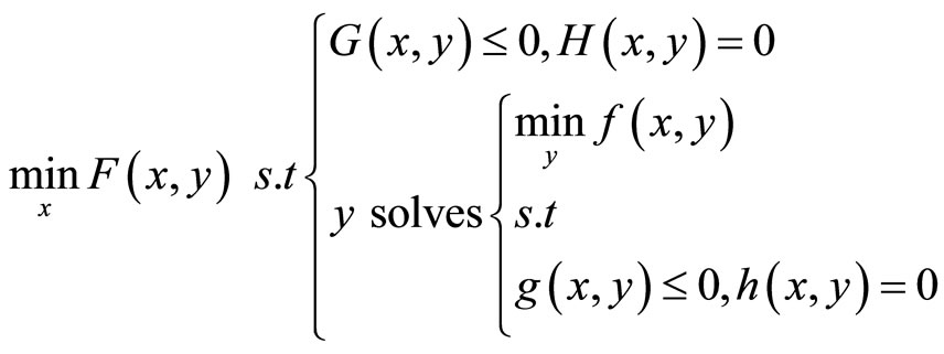
where:

With

For fixed, the problem:

is called the lower level or the follower problem parameterized by x. F and f are respectively the leader (or higher level) and the follower (or lower level) objective functions. G and H (respectively g and h) are leader’s inequality and equality constraints (respectively follower’s inequality and equality constraints) functions.

If then, the functions F and f are scalar valued; meaning that the higher and lower level decision makers are optimizing each only one objective. This class of problems is called bilevel single objective optimization problems, or simply bilevel optimization problems. Bilevel optimization is an important research area since about three decades and there exists a huge quantity of studies related to that class of problems (see for example the book [3] and bibliography reviews [4-6]).

If and/or, then leader and/or follower objective functions are vector valued. We obtain a more general problem called bilevel multiobjective optimization problem (BMOP). In this case, the upper level decision maker and/or the lower level one are optimizing more than one (in general conflicting) objective simultaneously. This class of optimization problems has not yet received a broad attention in the literature and there are only few studies in the literature dealing with it (see for example [7-11]). According to Pieume et al. [12], this issue can be explained by at least three reasons: The difficulty of searching and defining optimal solutions; the lower level optimization problem has a number of tradeoff optimal solutions; and it is computationally more complex than the conventional multiobjective programming problem or a bilevel programming problem.

We are interested in this paper in establishing optimality conditions in bilevel multiobjective optimization, in the general case were both the higher and the lower level problems are multiobjectives. Inspired by optimality conditions given by A. A. K. Majumdar in [13] and D. S. Kim et al. [14] for (single level) multiobjective optimization problems (MOP), we established new sufficient optimality conditions for a solution of a general BMOP with coupled upper level constraints. To our knowledge, there are very few studies in the literature dealing with optimality conditions in bilevel multiobjective programming. In [7], using the Kunh Tucker conditions for MOP, A. Dell’Aere stated a necessary condition for solution of a BMOP in the case where lower level inequality constraints are absent. Jane J. Ye presented in [15] for bilevel programs in which only the leader problem is vector valued, necessary optimality conditions in the case where the Karush-Kuhn-Tucker (KKT) condition is necessary and sufficient for global optimality of all lower level problems near the optimal solution, by replacing the lower level problem by its KKT conditions. In the case where the KKT conditions are not necessary and sufficient for global optimality, she derives necessary optimality conditions by considering a combined problem where both the value function and the KKT conditions of the lower level problem are involved in the constraints. More recently, S. Dempe et al. in [16] presented for the optimistic formulation of a bilevel optimization problem with multiobjective lower-level problem, necessary optimality conditions by considering the scalarization approach for the lower level multiobjective program and transforming the problem into a scalar-objective optimization problem with inequality constraints by means of the optimal value reformulation.

The rest of the paper is organized as follows: In the next section, definition of solution concepts and characterization of bilevel multiobjective programming problems are presented. In Section 3, after presenting some preliminary notions, we present sufficient optimality conditions for a solution of BMOP; the paper is concluded in Section 4.

2. Definition and Characterization of Bilevel Multiobjective Programming Problems

Let and be two vectors of,. The following ordering relations (in) will be used:

We consider the following problem:

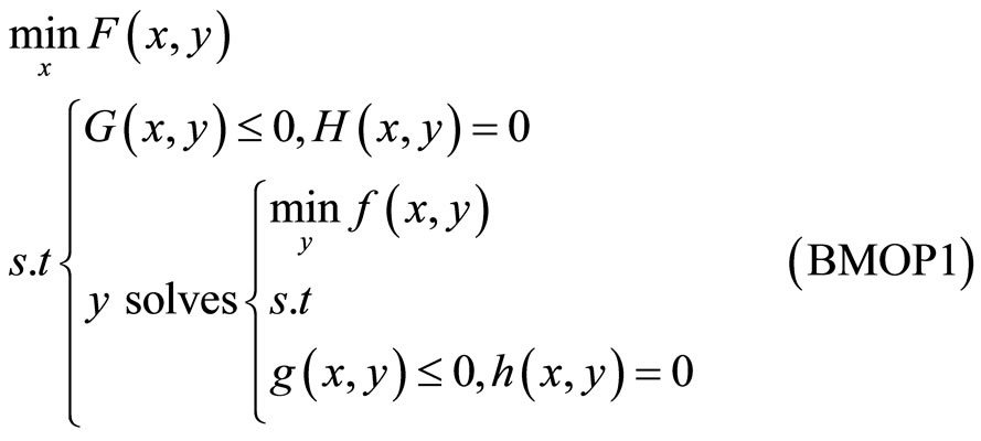
where:

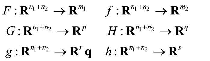
With and since, the problem is a Bilevel Multiobjective Optimization Problem (BMOP).

For all, let:

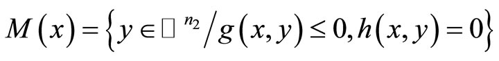
For all, let:

For all, let:

● 

●  is the set of the pareto optimal solutions of the follower’s problem parameterized by.

●  is the set of weak pareto optimal solutions of the follower’s problem parameterized by.

Definition 2.1. is said to be a solution of BMOP1 if and only if, and there exists no, such that

.

Definition 2.2. is said to be a weak solution of BMOP1 if and only if, and there exists no, such that.

Let’s consider a BMOP with uncoupled upper level inequality constraints and without equality constraints in both levels:

Then under the strict convexity of the upper and lower level objective and constraints functions, the definition 2.1 of a solution of a Bilevel Multiobjective Optimization problem is equivalent to the following conditions:

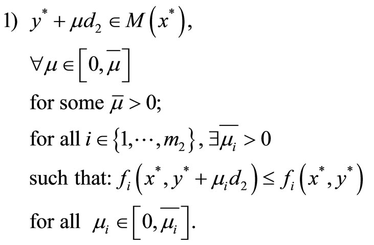
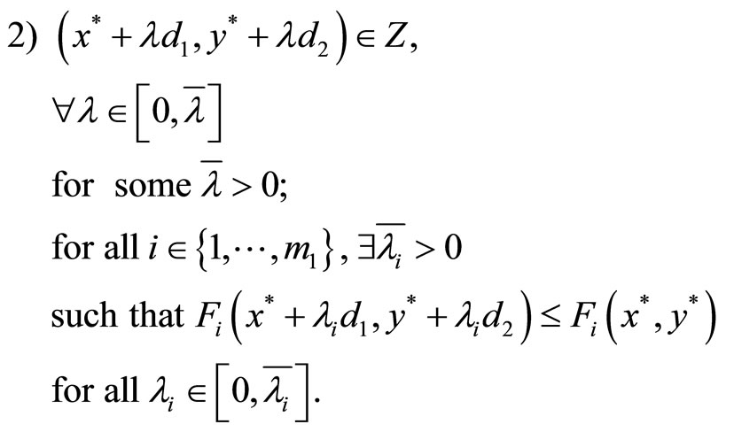
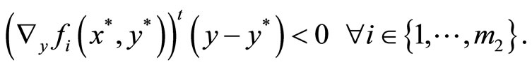
Theorem 2.1. Assume that F and G are strictly convex, and that, are strictly convex. Then, is a solution of (BMOP2) if and only if there are no directions such that:

Proof

Suppose that is a solution of (BMOP2). We have to prove that satisfying 1) and 2) don’t exist.

To the contrary, suppose that exist.

Let.

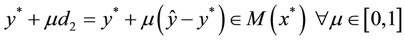
Define; Take

.

Since (according to 1).

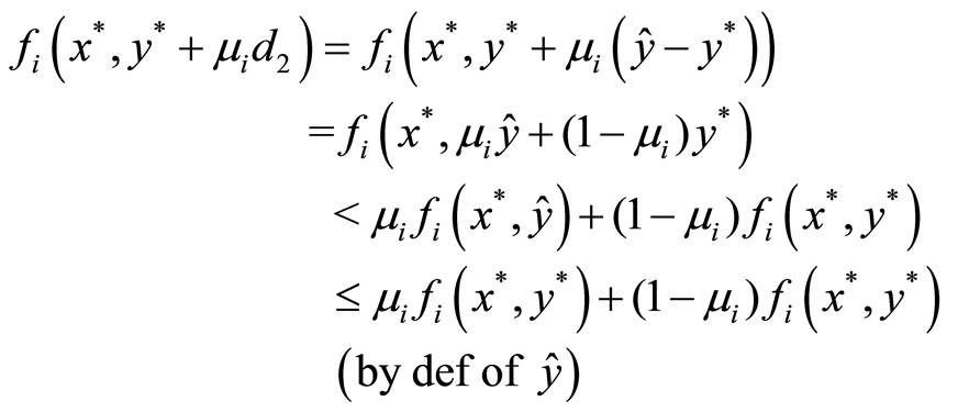
By definition,. Using the strict convexity assumption on f, we have:

That is; this implies that.

Hence; which contradicts the fact that is a solution of (BMOP2).

Suppose that don’t exist. Let’s prove that is a solution of (BMOP2).

To the contrary, suppose that is not a solution of (BMOP2). Then or

and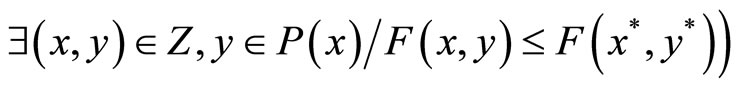

● Suppose that.

Then,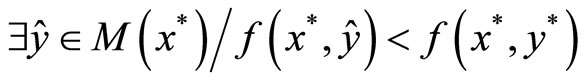

Define.

Since is convex, is convex.

By the convexity of, we have

.

Let and fixed.

Hence there exist satisfying 1), which is a contradiction with the hypothesis.

● Suppose that and

Let.

(by the convexity of Z).

Let and arbitrary fixed.

Hence there exist satisfying 2); which contradict the hypothesis.

The main difficulty when solving a BMOP comes from the fact that for each feasible alternative x, the leader must know exactly, in order to take his decision, what will be the reaction of the lower level decision maker. But since the lower level problem is a multiobjective one, for each leader’s alternative x, the follower has many (sometimes infinite) possible responses, which are represented by the entire follower pareto optimal set P (x). To circumvent this difficulty, there are rational reformulations of the problem, which really speaking are relaxations of the BMOP. They are: The optimistic or risky formulation, the pessimistic or conservative formulation, the mean formulation and the stochastic formulation.

Definition 2.3.

1) Optimistic or risky formulation of a BMOP

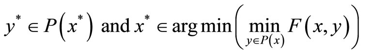
An optimistic or risking leader always chooses for all feasible alternative x, the follower Pareto optimal solution which satisfy his objective (in the sense of minimization).

is said to be an optimistic optimal solution of a BMOP if and only if

2) Pessimistic or conservative formulation of a BMOP

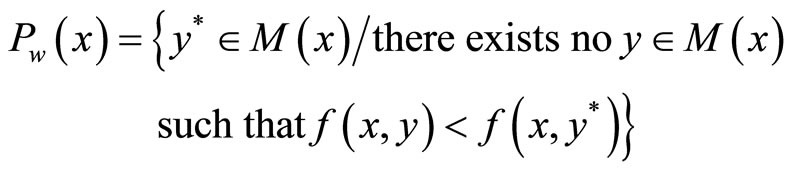
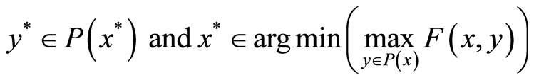
A conservative or pessimistic leader always prefer to choose for all feasible alternatives x, the follower pareto optimal solution which is the worse for him (in the sense of minimization).

said to be a pessimistic optimal solution of a BMOP if and only if

3) Mean formulation of a BMOP

Suppose that and that for all is integrable on.

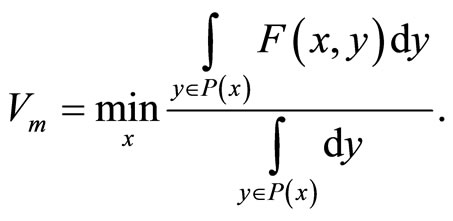
A mean leader always chooses the mean solution among the follower pareto optimal solutions, for each feasible higher level decision x.

is said to be a mean optimal solution of a BMOP if and only if

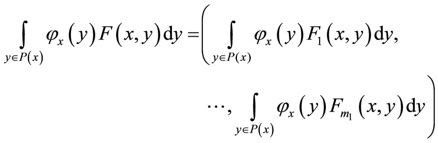
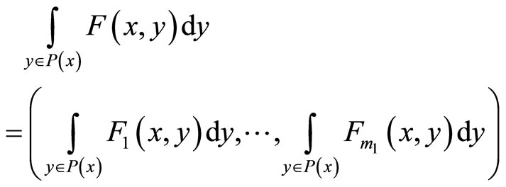
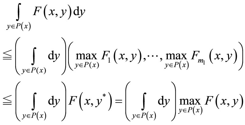
where since F is a vector valued function, we define its integral over by:

4) Stochastic formulation of BMOP

Suppose that for all leaders’ alternative x, there exists a probability distribution with as density function such that the leader always has the probability to choose y as the follower reaction among his pareto optimal solution set. Then, one can talk of a stochastic formulation of the BMOP.

is said to be a stochastic optimal solution of the BMOP if and only if

where:

When there exists a unique solution to the lower level problem for any x, the above mentioned solutions are not different. But when there are multiple solutions to the lower level problem, the four kinds of solutions are different.

There exists a relationship between the four types of solutions. In [17], a theorem giving the relationship between the optimistic optimal value, pessimistic optimal value and mean optimal value, in case where only the lower level problem is multi-objective is presented and proved.

The following proposition generalize the above mention theorem (theorem 0.5 in [11]) to the general case where both upper and lower level problems are multiobjective.

Proposition 2.1.

Denote as optimistic optimal value, pessimistic optimal value, mean optimal value and stochastic optimal value of BMOP1 respectively. Then, we have: and.

Where “” is the partial order defined above.

Proof

1) Let x be a feasible alternative of the leader. By definition,

For all, we have

hence

(1)

Let

(1)

Then

Hence

2) By a similar reasoning as in 1), we obtain that

Hence by the transitivity of “”.

The proof of the second relation is analogous while using the fact that.

3. Suffcient Optimality Conditions for a Solution of BMOP

3.1. Preliminary Definitions

Definition 3.1. Quasiconvexity, strict quasiconvexity, pseudoconvexity, strict pseudoconvexity ([18])

Let 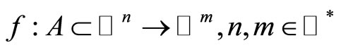and.

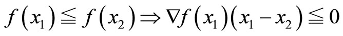
1) f is said to be quasiconvex at (with respect to A) if:

if in addition f is differentiable, then we have the following equivalent definition:

f is quasiconvex if for all

2) f is said to be strictly quasiconvex at (with respect to A) if:

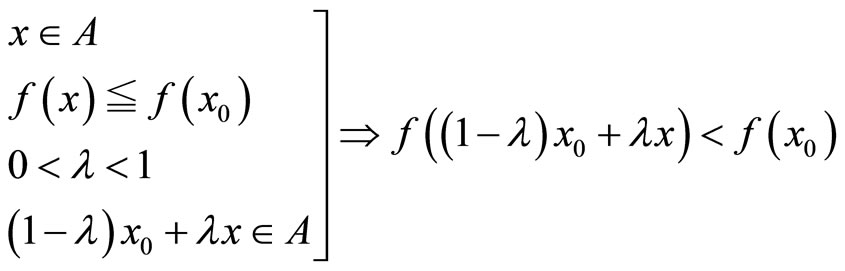
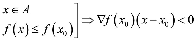
3) f is said to be pseudoconvex at (with respect to A) if it is differentiable and

or

4) f is said to be strictly pseudoconvex at (with respect to A) if it is differentiable and

We have the following implications [18]:

strict convexity convexity strict pseudoconvexity pseudoconvexity strict quasiconvexity quasiconvexity.

3.2. Sufficient Optimality Conditions

We consider the problem BMOP1.

For fixed, let,

.

Let;

be respectively the sets of active inequality constraints of the follower and leader at respectively.

Theorem 3.1.

Let.

Suppose the following:

1) is pseudoconvex at; F is pseudoconvex at.

2) and are quasiconvex and differentiable at; and H are quasiconvex and differentiable at.

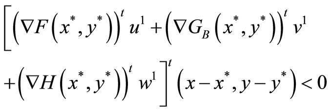
3) There exists and such that:

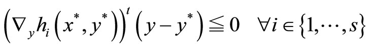
a)

b)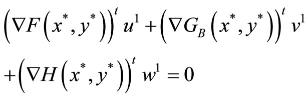

Then, is a weak solution of BMOP1.

Proof

Let verifying 1), 2) and 3).

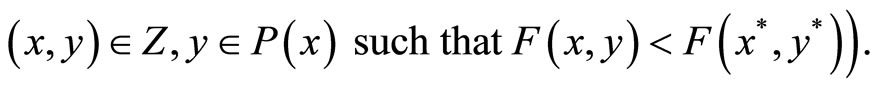
Suppose that is not a weak solution of BMOP1.

Then, or

1) Suppose that.

Then, such that i.e. such that

By the pseudoconvexity of, we have:

(1)

Let be arbitrary fixed.

Then, it holds from (1) that:

(2)

We have:

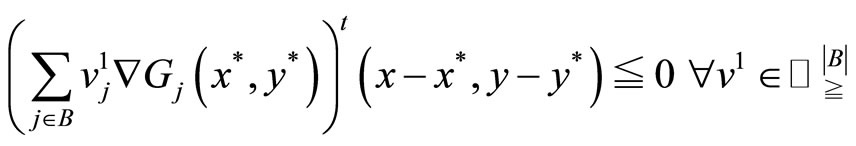
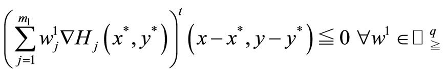
By the quasiconvexity and differentiability assumption in assertion 2) of the theorem, we have:

(3)

(4)

Let and be arbitrary fixed.

Then it holds from (3) and (4) that:

(5)

(6)

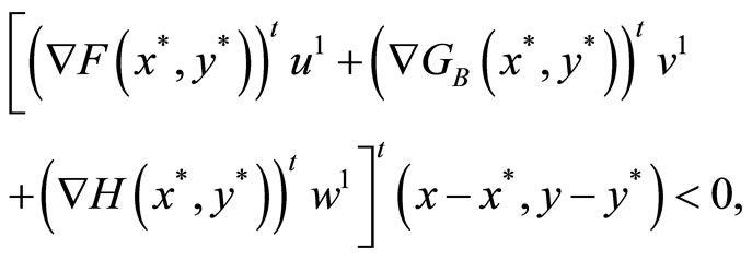
From (2), (5) and (6), we have:

with arbitrary fixed.

i.e. we have:

with arbitrary fixed; which violates the assumption 3) a) of the theorem.

2) Suppose that

By the same way of reasoning as in the first case, we obtain:

It holds from the linearity of the scalar product that:

With arbitrary fixed.

This violates the assumption 3) b) of the theorem.

Conclusion: is a weak solution of BMOP1.

A suffcient optimality condition for a solution of BMOP1 is obtained by replacing the pseudoconvexity of the upper and lower level objective function by the strict pseudoconvexity.

Theorem 3.2.

Let.

Suppose the following:

1) is strictly pseudoconvex at; F is strictly pseudoconvex at.

2) and are quasiconvex and differentiable at; and H are quasiconvex and differentiable at.

3) There exists and such that:

a)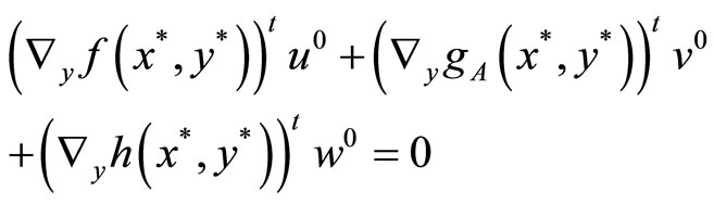

b)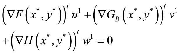

Then, is a solution of BMOP1.

Proof

Let verifying 1), 2) and 3).

Suppose that is not a solution of BMOP1.

Then or

1) Suppose that; then such that. By the strict pseudoconvexity of we have:

by a reasoning similar to that used in the proof of theorem 3.1. we obtain:

; which contradicts the assumption 3) a) of the theorem.

2) Suppose that

By the strict pseudo convexity of F, we have:

Using a similar reasoning to that used in theorem 3.1, we obtain:

;

which violates the assumption

3) b) of the theorem.

Conclusion: is a solution of BMOP1.

As corollaries of theorem 3.1 and theorem 3.2, we obtain the following sufficient optimality theorems:

Corollary 3.1.

Let.

Suppose the following:

1) and are convex and differentiable at.

2) F, G and H are convex and differentiable at.

3) There exists and

such that:

c)

d)

Then, is a weak solution of BMOP1.

Corollary 3.2.

Let.

Suppose the following:

1) and are strictly convex and differentiable at.

2) F, G and H are strictly convex and differentiable at.

3) There exists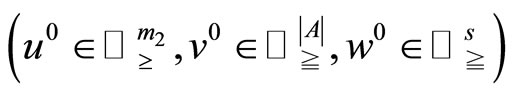 and

such that:

a)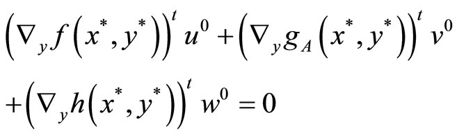

b)

Then, is a weak solution of BMOP1.

The corollaries 3.1 and 3.2 can be proved in two ways; either analogously to the proofs of theorem 3.1 and 3.2 or using the fact that: Strict convexity convexity strict pseudoconvexity pseudoconvexity strict quasiconvexity quasiconvexity.

4. Conclusion

In this paper, we have established new sufficient optimality theorems for a solution of a differentiable bilevel multiobjective programming problem. We have also presented a result giving a relationship between the optimistic optimal value, the pessimistic optimal value and the mean optimal value (respectively the stochastic optimal value) of a BMOP. The latter result shows that the mean formulation and the stochastic formulation can be very useful in practice to compute good approximations of the solution set of a BMOP in which the follower is not supposed to always report worst cases (in the leader’s point of view)¹ nor to react in a way which will lead to the leader’s goal attainment². Therefore, investigating these two formulations of a BMOP might be interesting for future research.

REFERENCES

NOTES

¹This is the case where the pessimistic formulation is the most adequate.

²This is the case where the optimistic formulation is the most suitable.

REFERENCES

- H. Von Stackelberg, “The Theory of Market Economy,” Oxford University Press, Oxford, 1952.
- P. Heiskanen, “Decentralized Method for Computing Pareto Solutions in Multiparty Negotiations,” European Journal of Operational Research, Vol. 117, No. 3, 1999, 578- 590. doi:10.1016/S0377-2217(98)00276-8
- S. Dempe, “Foundations of Bilevel Programming,” Kluwer Academic Publisher, Dordrecht, 2002.
- S. Dempe, “Annotated Bibliography on Bilevel Programming and Mathematical Programs with Equilibrium Constraints,” Optimization, Vol. 52, No. 3, 2003, pp. 333- 359. doi:10.1080/0233193031000149894
- L. N. Vicente and P. H. Calamai, “Bilevel and Multilevel Programming: A Bibliography Review,” Journal of Global Optimization, Vol. 5, No. 3, 1994, pp. 291-306. doi:10.1007/BF01096458
- B. Colson, P. Marcotte and G. Savard, “An Overview of Bilevel Optimization,” Annals of Operational Research, Vol. 153, No. 1, 2007, pp. 235-256.
- A. Dell’Aere, “Numerical Methods for the Solution of Bi-Level Multi-Objective Optimization Problems,” Ph.D. Thesis, University of Paderborn, Paderborn, 2008.
- K. Deb and A. Sinha, “Solving Bilevel Multi-Objective Optimization Problems Using Evolutionary Algorithms,” Technical Report KanGAL Report No. 2008005, Indian Institute of Technology, Kanpur, 2008.
- C. O. Pieume, L. P. Fotso and P. Siarry, “Solving Bilevel Programming Problems with Multicriteria Optimization Techniques,” OPSEARCH, Vol. 46, No. 2, 2009, pp. 169- 183.
- G. Eichfelder, “Multiobjective Bilevel Optimization”, Mathematical Programming, Vol. 123, No. 2, 2008, pp. 419- 449. doi:10.1007/s10107-008-0259-0
- G. Eichfelder, “Solving Nonlinear Multiobjective Bilevel Optimization Problems with Coupled Upper Level Constraints,” Technical Report Preprint No. 320, PreprintSeries of the Institute of Applied Mathematics, University Erlangen-Nürnberg, Erlangen and Nuremberg, 2007.
- C. O. Pieume, P. Marcotte, L. P. Fotso and P. Siarry, “Solving Bilevel Linear Multiobjective Programming Problems,” American Journal of Operations Research, Vol. 1 No. 4, 2011, pp. 214-219.
- A. A. K. Majumdar, “Optimality Conditions in Differentiable Multiobjective Programming,” Journal of Optimization Theory and Applications, Vol. 92, No. 2, 1997, pp. 419-427. doi:10.1023/A:1022667432420
- D. S. Kim, G. M. Lee, B. S. Lee and S. J. Cho, “Counterexample and Optimality Conditions in Differentiable Multiobjective Programming,” Journal of Optimization Theory and Applications, Vol. 109, No. 1, 2001, pp. 187-192. doi:10.1023/A:1017570023018
- J. J. Ye, “Necessary Optimality Conditions for Multiobjective Bilevel Programs,” Journal of the Institute for Operations Research and the Management Sciences, Vol. 36, No. 1, 2010, pp. 165-184.
- S. Dempe, N. Gadhi and A. B. Zemkoho, “New Optimality Conditions for the Semivectorial Bilevel Optimization Problem,” Journal of Optimization Theory and Applications, Published online, August 2012.
- P.-Y. Nie, “A Note on Bilevel Optimization Problems,” International Journal of Applied Mathematical Sciences, Vol. 2, No. 1, 2005, pp. 31-38.
- O. L. Mangasarian, “Nonlinear Programming,” Mc GrawHill Book Company, New York, 1969.
NOTES
1This is the case where the pessimistic formulation is the most adequate.
2This is the case where the optimistic formulation is the most suitable.