Abstract

This paper provides a methodology for valuing a Loan Credit Default Swap Index (LCDX) and its tranches involving both default and prepayment risks. The valuation is path dependence, where interest, default and prepayment rates are correlated stochastic processes following CIR processes. By Monte Carlo simulation, a numerical solution and team structure of tranched LCDX are obtained. Computing examples are provided.

1. Introduction

Credit markets have seen an explosive growth over the last decade. New products, like CDOs, CPDOs, are brought to the market with an unprecedented complexity. However, the financial crisis happened three years ago makes people more careful with these products.

Loan-only Credit Default Swaps, called LCDS in simple, are financial instruments that provide the buyer an insurance against the default of the underlying syndicated secured loan. Its markets were launched in 2006 both in US and Europe. It can be seen that there is an explosive growth of the markets these years. Comparing to a standard Credit Default Swaps (CDS), a LCDS contract is almost the same, except that 1) its reference obligation is limited on loans; 2) it can be cancelled. So that, the pricing of LCDS must take into account not only default probabilities with recovery rate, but also the prepayment probabilities. These two probabilities are negative correlated. The stronger the relationship between default and prepayment, the higher the LCDS spread.

Like a CDS Index (CDX), a Loan Credit Default Swap Index (LCDX) is the most popular index of LCDSs and is composed of 100 equally weighted single-name LCDSs. It is the benchmark index for the loan-only CDS in North America. LCDX was the first standardized liquid product for taking directional views on a portfolio representing the syndicated secured loan market. Moreover, positions can be taken by now in standardized tranches on LCDX: [0% - 5%], [5% - 8%], [8% - 12%], [12% - 15%] and [15% - 100%]. The [0% - 5%] tranche is quoted as upfront premium (no running spread), while the other tranches are quoted in running spread. LCDS trades are cancelable if no suitable debt remains to deliver upon settlement. The LCDS trades are then completely canceled and the corresponding LCDX trades are factored down. LCDX tranches are affected by simply reducing the size from the super-senior tranche because of prepayment, while the most junior tranche is reduced by default of the reference first as CDX.

In the literature, different models for pricing risk derivatives. These models can be classified into two main categories known as structural and reduced form models. Structural models are based on the model proposed by Merton [1], which shows that a company’s equity can be regarded as European call options. Black-Cox [2], and Longstaff and Schwartz [3] developed the model for default event as soon as the firm’s asset value falls below a certain level. Reduced form models are not determined by the firm value, but by the first jump of an exogenous jump process. The parameters governing the default hazard rate are inferred from market data. These models can incorporate correlations between defaults by allowing hazard rates to be stochastic and correlated with macroeconomic variables. Duffie and Singleton [4], Lando [5], and Zhou [6] provide examples of research using this approach. For the pricing LCDS, Zhen Wei [7] considered a single name LCDS, where default and prepayment intensities were involved. He used a single-factor model with common factor and correlation coefficient to depict the negative relationship between default and prepayment, whose rates follow double stochastic process. However, his model allows a negative prepayment rate, which lacks of financial meaning. Based on Zhen Wei’s work, Dobranszky et al. [8] times the prepayment intensity with a coefficient variation to describe the relationship between LCDS and CDS.

For pricing a basket LCDS, the reduced form model is used more frequently due to the scale and complexity of the pool. The reduced form model can be classified to two categories: “bottom up” and “top down”. In a bottom up model, the portfolio intensity is an aggregate of the constituent intensities. In a top down model, the collateral portfolio is modeled as a whole, instead of drilling down to individual constituents; the portfolio intensity is specified without reference to the constituents. The constituent intensities are recovered by random thinning. The benefit of a top-down approach is its simplicity as a result of not having to model the individual constituents of the underlying portfolio. Giesecke [9] contrasts these two modeling approaches. It emphasized the role of the information filtration as a modeling tool. Wu, Jiang and Liang [10] use top-down model to pricing of MBS with repayment risk. Using bottom upframework, Shek, Uematsu and Zhen Wei [11] studied pricing a CDS referenced a pool loan, described the default and prepayment by single-factor Gaussian Copula model. They obtained the spread of the LCDX through Monte Carlo simulation. Dobranszky and Schoutens [12] used single-name copula to describe the relationship between default and prepayment. Under “top down” and intensity framework, Liang and Zhou [13] using a single-factor model, correlated default and prepayment risks are considered, where they are considered as two kinds of decreases in the pool, and the stochastic interest rate is used to be their common factor, where negative intensity of prepayment is described as refinance. A closed form solution is obtained in the work.

In this paper, we deal with structured credit risk products quite similar to the synthetic CDO of credit default swaps (CDS). More precisely, a tranched portfolio of loan-only credit default swaps (LCDS) is considered. Under “top down framework”, and based on work of [8], the references pool of LCDX is considered as an entity. The difficulty here is that the default and prepayment are negative correlated and affect LCDX in different directions and they are path dependent as ones of an Asian option. That means, the pricing has no analytical solution. By linear transformation, we use independent random variables to express interest, default and prepayment rates. Through Monte Carlo simulation, we obtain numerical solutions. Numerical examples are presented.

The structure of the paper is as follows: In the next section, we establish a pricing model for LCDX, by introducing two processes of default and prepayment rates. In the third section, we use CIR processes to describe interest, default and prepayment rates, then the pricing model can be calculated. In the fourth section, some numerical examples are shown. Summary is in the Conclusion section.

2. Modeling LCDX

As mentioned before, the main point of LCDS is a probability that the loan prepays earlier and hence the instrument is cancelable. During the life of an LCDS contract, two kinds of events may be triggered, either the underlying loan is prepaid or the loan-taker goes to default. If a prepayment event were triggered first, the LCDS would have been cancelled. Otherwise, the LCDS would have defaulted, when the LCDS issuer would have to pay the recovery adjusted notional amount to the LCDS buyer.

On the model established in LCDS [13] at time s, , where and are the accumulative amount of default prepayment respectively, and is the outstanding principal balance at time s. Then for any s > 0,

The default and prepayment risks have opposite impact on the tranches. The default goes from the junior-most tranche until it is completely redeemed, then allocated to the next tranche, while the prepayment goes from the senior-most tranche until it is completely redeemed. The prepayment does not result in loss, thus the investor need not pay for prepayment.

Denoted the accumulative loss in the pool at time s by. For a mezzanine tranche [A,B], (0 ≤ A ≤ B ≤ 1) with attachment point A and detachment point B, we define its accumulative loss at time s as:

It can also be expressed as

The accumulative decrease on the notional principal at time s is

(1)

The second term in the right side of (1) is coming from the fact that defaults amortize the senior-most tranche. Hence, when defaults occur, both the junior-most and the senior-most tranches are impacted. The junior-most tranche notional principal is reduced by the amount of the loss and the senior-most tranche notional principal is amortized by the amount of the recovery. We define the decrease on the notional principal of the tranche [A, B] at time s as:

The fair spread of tranche [A, B] is chosen such that the expected present value of the fee payments for that tranche is equal to the expected loss payments.

The fee payment can be calculated as

and the expected loss payment is shown as

Then c is chosen such that it balances and, i.e.

(2)

This is the pricing formula for tranched LCDX.

3. The Solution Under CIR Process

In [13], we use a single-factor model to describe the relation between default and prepayment. By this model, we can find an affine solution for LCDS. When pricing LCDX, the pricing Equation (2) is much more complicated than the one of LCDS. The model in LCDX turns to path dependent, somewhat like the ones of arithmetic average options. Therefore, using the single-factor model, the problem cannot be simplified. Thus, in this study, we use CIR Process to describe the behavior and correlation of, and directly. This is also guaranteed that all rates are positive. By Monte Carlo simulation, we obtain a numerical spread solution.

Suppose that, and follows the stochastic process of CIR, i.e.

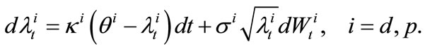
Rewrite the formula as

(3)

where κ, θ, σ etc. are all positive constants;, and follow standard Brown Motion. It is well know that, under the condition

These CIR processes are nonnegative and their boundaries at origin are unattainable [14,15].

These three processes are correlated. Denoted, by the correlations of, and respectively. As the default and prepayment rates are opposite correlated to the interest rate, the first one is positive while the second one is negative. That means,. No matter how interest rate changes, the relationship of the default and the prepayment rates is negative, i.e..

The covariance matrix is denoted by is:

To fetch random numbers which are not independent for a simulation, we need to deal with the correlation of the variables. Here, we introduce a lemma:

Lemma A linear transformation of a normal distribution is still a normal one.

According to this theorem, we can find an independent process vector, a 3 × 3 matrix A and three-dimension constant vector b such that

(4)

where

Take Equation (4) into (3), we have,

(5)

where

After transformation, the correlated variables are expressed as independent ones. Now, we can establish a process of the numerical calculation: First, we simulate three paths of independent Brown Motion. Second, taking them into Equation (5), we obtain the paths of interest rate, default rate and prepayment rate. Third, taking these into pricing Equation (2), by difference method, we obtain the price of different trances. This result can be treated as random samples of all the possible prices. Another path can get another random sample. At last, repeating this process thousands of times, getting an assemble of price, averaging these random samples, we can obtain the final price of each tranche of LCDX.

4. Numerical Examples

So far, we have derived the pricing Equation (2) and numerical method. Here, we give some examples.

Now, take t = 0, R = 0.3, and consider the spread of LCDX.

Figure 1 shows the shape of LCDX term structures with

The graph shows that the spread curves of different tranches are not intersected. That because that the default and prepayment start from the junior-most and seniormost tranches first respectively. They allocate next tranches only the present ones completely redeemed. It also can be seen that the spread of senior-most tranche is very low and close to 0, which is the manifestation of taking default risk last and prepayment first.

The shape of curve [5% - 8%] is steep during time 2.5 and 5 which implies that the default is larger. The curve becomes horizontal from time 8 which indicates that the accumulated loss is beyond of this tranche, and the default is already allocated to the next tranche.

Figure 2 shows a three dimension figure of tranche spread [5% - 10%] with respect to the initial values of default and prepayment rates at time 4. If the initial value of default goes up, which means the probability of default goes larger as well, it results that the spread is more expensive. On the contrary, if the initial value of prepayment goes up, which means the probability of prepayment goes larger, it is an advantage for the investor of this tranche and results that the spread is cheaper.

Figure 3 shows the impact of correlations. In the graph, ρ ≠ 0 means that , while ρ = 0 means. Whichever tranche, the two curve are very close, which manifests that the correlation have little impact on tranche spread. The division of asset pool into several tranches redistributes the investment returns and risks. It also reduces the impact of correlation between variables on spread.

Figure 4 shows the impact of two parameters on a junior tranche: mean reversion rate and long-term-mean of the default rate, since default starts from the senior-most tranche. Here, the tranche [5% - 8%] is considered. The spread increases as the mean reversion increases. In our example, as the mean is bigger than initial value, the default rate reverses upward. That means, the greater the reversion, the larger the probability of default is. This results that the

spread is more expensive. The increasing of long-term implies the increasing the spread.

Figure 5 shows that the impact on a senior tranche of mean reversion rate and long-term-mean of prepayment rate, since prepayment starts from the senior-most tranche. Here, tranche [12% - 15%] is chosen. The spread deceases as the mean reversion increases. In our example, as the mean is bigger than initial value, the prepayment rate reverse upward. The greater the reversion, the larger the probability of prepayment is, which results that the spread is cheaper. The increasing of long-term mean also causes the spread decease.

5. Conclusions

We establish a model for pricing LCDX under the reduced form framework, where the default and prepayment rates are correlated with interest rate. All these rates are assumed follow CIR process. Using Monte Carlo method, we obtain numerical solution and term structure of tranched LCDX with graphs, by which parameter analysis are carried on.

6. Acknowledgements

This work is supported by National Basic Research Program of China (973 Program) 2007CB814903.

7. References

[1]       R. Merton, “On the Valuation of Corporate Debt: the Risk Structure of Interest Rates,” Journal of Finance, Vol. 29, No. 2, 1974, pp. 449-470. doi:10.2307/2978814

[2]       F. Black and J. Cox, “Valuing Corporate Securities: Some Effects of Bond Indenture Provisions,” Journal of Finance, Vol. 31, No. 2, 1976, pp. 351-367. doi:10.2307/2326607

[3]       F. Longstaff and E. Schwartz, “A Simple Approach to Valuate Risky Fixed and Floating Rate Debt,” Journal of Finance, Vol. 50, No. 3, 1995, pp. 789-819. doi:10.2307/2329288

[4]       D. Duffie and K. J. Singleton, “Modeling Term Structure of Defaultable Bonds,” Review of Financial Studies, Vol. 12, No. 4, 1999, pp. 687-720. doi:10.1093/rfs/12.4.687

[5]       D. Lando, “On Cox Processes and Credit Risky Securities,” Review of Derivatives Research, Vol. 2, No. 2-3, 1998, pp. 99-120. doi:10.1007/BF01531332

[6]       C. Zhou, “An Analysis of Default Correlation and Multiple Defaults,” Review of Financial Studies, Vol. 14, No. 2, 2001, pp. 555-576. doi:10.1093/rfs/14.2.555

[7]       W. Zhen, “Valuation of Loan CDS under Intensity Based Model,” Working Paper, Stanford University, 2007.

[8]       P. Dobranszky, “Joint Modeling of CDS and LCDS Spreads with Correlated Default and Prepayment Intensities and with Stochastic Recovery Rate,” Technical Report 08-04, Section of Statistics, Leuven, 2008.

[9]       K. Giesecke, “Portfolio Credit Risk: Top Down vs. Bottom Up Approaches,” In: R. Cont, Ed., Frontiers in Quantitative Finance: Credit Risk and Volatility Modeling, John Wiley & Sons, Chichester, 2008.

[10]    S. Wu, L. S. Jiang and J. Liang, “Pricing of MortgageBacked Securities with Repayment Risk,” Working Paper, 2008.

[11]    H. Shek, S. Uematsu and W. Zhen, “Valuation of Loan CDS and CDX,” Working Paper, Stanford University. 2007.

[12]    P. Dobranszky and W. Schoutens, “Generic Levy OneFactor Models for the Joint Modeling of Prepayment and Default: Modeling LCDX,” Technical Report 08-03, Section of Statistics, Leuven, 2008.

[13]    J. Liang and Y. J. Zhou, “Valuation of a Basket Loan Credit Default Swap,” International Journal of Financial Research, Vol. 12, 2010, pp. 21-29.

[14]    L. S. Jiang, “Mathematical Modeling and Cases Analysis of Financial Derivative Pricing,” Higher Education Press, Beijing, 2008.

[15]    V. Linetsky, “Computing Hitting Time Densities for CIR and OU Diffusions: Applications to Mean-Reverting Models,” Journal of Computational Finance, Vol. 7, No. 4, 2004, pp. 1-22.