ABSTRACT

As much as accurate or precise position estimation is always desirable, coarse accuracy due to sensor node localization is often sufficient. For such level of accuracy, Range-free localization techniques are being explored as low cost alternatives to range based localization techniques. To manage cost, few location aware nodes, called anchors are deployed in the wireless sensor environment. It is from these anchors that all other free nodes are expected to estimate their own positions. This paper therefore, takes a look at some of the foremost Range-free localization algorithms, detailing their limitations, with a view to proposing a modified form of Centroid Localization Algorithm called Reach Centroid Localization Algorithm. The algorithm employs a form of anchor nodes position validation mechanism by looking at the consistency in the quality of Received Signal Strength. Each anchor within the vicinity of a free node seeks to validate the actual position or proximity of other anchors within its vicinity using received signal strength. This process mitigates multipath effects of radio waves, particularly in an enclosed environment, and consequently limits localization estimation errors and uncertainties. Centroid Localization Algorithm is then used to estimate the location of a node using the anchors selected through the validation mechanism. Our approach to localization becomes more significant, particularly in indoor environments, where radio signal signatures are inconsistent or outrightly unreliable. Simulated results show a significant improvement in localization accuracy when compared with the original Centroid Localization Algorithm, Approximate Point in Triangulation and DV-Hop.

Keywords:

Anchors, Centroid Localization Algorithm (CLA), Wireless Sensor Networks, Received Signal Strength (RSS), Range-Free, Reach Centroid Localization Algorithm (ReachCLA)

1. Introduction

Localization is determining the position of a device or a node, relative or absolute with an appropriate accuracy [1] . Localization is an implicit bargain in wireless sensor networks. The inherent characteristics of these sensor networks make a node’s location an important part of their state [2] . Irrespective of the fundamental objective of sensing or monitoring, whether for disaster monitoring, target tracking, intrusion detection or climate reporting, localization remains an inherent capability of wireless sensor networks (WSN).

WSN devices remain a highly promising alternative to Global Positioning Systems (GPS) for location estimation, particularly indoors where GPS signals are unavailable [3] . Location of sensor nodes can be obtained either by using sensor nodes of known geographical coordinates, called anchors, or by using GPS enabled sensors as anchors. In applications requiring knowledge of global coordinate systems, the anchors determine the location of sensor nodes with reference to the global coordinate system and the application where a local coordinate system is sufficient, the position of sensor nodes is referred to as the local coordinate system of the network [4] .

The problem with the later is two-fold; cost of deployment of the anchors will be high and deploying such anchors indoors will be unproductive due to line of sight limitations of GPS devices. A major advantage of WSN devices in this regard is their ease of deployment; they are fault tolerant, and could avail themselves high levels of connectivity in close clusters. They are miniaturized and are comparatively of low cost. However, energy consumption becomes a key concern in order to assure availability, particularly for reliable localization to be available [5] .

Localization accuracy and reliability are dependent on node density, as connectivity information is more reliable when sensors are in close proximity to each other. High node density in sensor networks prevents them from being completely remote or isolated from every other node. Therefore, in a dense WSN, sensor nodes are expected to be highly connected.

Many localization algorithms have been proposed for location estimation. However, localization algorithms can be classified into two categories; Range- based [2] [3] [4] [5] [6] and Range-free algorithms [7] [8] .

Range-based algorithms use absolute point-to-point estimation techniques using either distance or angle for range estimation. These techniques require the installation of precision and costly hardware such as directional antennas for distance estimation [9] [10] . In Range-based techniques, distance estimation is achieved by using one of the following techniques: Time of Arrival (ToA), Time difference of Arrival (TDoA), Angle of Arrival (AoA) [11] or Received Signal Strength (RSS) [12] . Location discovery happens in two phases using any of these techniques: ranging phase and estimation phase.

The ranging phase can also be referred to as estimation phase. Here, each free node approximates its distance or angle from its neighbours. At the estimation phase or distance combination phase, the free nodes use ranging information of the anchor nodes to estimate their own position [13] [14] .

Range-free algorithms explore connectivity information between adjacent nodes. They use unique protocols to eliminate the need for radio signal measurement. These classes of algorithm use radio communication range to establish the nodes that are within a particular communication sphere. They operate on the idea that once two nodes can communicate, then the distance between the nodes, within a certain probability, is less than their highest transmission range.

Unlike Range-based algorithms, Range-free algorithms do not rely on distance measurement and they also do not require extra hardware, hence, they are cost- effective. Range-free techniques explore the availability of radio signals for location estimation. Many Range-based localization algorithms propose solutions that are founded on impractical assumptions such as; assuming a uniform distribution of radio signals, symmetric radio connectivity between nodes, availability of additional hardware, lack of obstructions, the perpetual availability of line-of-sight, no multipath effects, and flat terrain.

Rang-free algorithms circumvent these assumptions as these classes of algorithms do not estimate the absolute point-to-point distance between anchors and sensors. The algorithm can be implemented on cheap sensors without the need for modification and the algorithm requires low computational power. However, most Range-free algorithms are proximity based algorithms, thus, they are likely to be less accurate than Range-based algorithms.

Enclosed geographical spaces further present more complex challenges to localization. More complex hardware integration would therefore be required for any Range-based WSN localization to be effective. Two major challenges that will be encountered when applying Range-based algorithms for indoor localization are multipath effects of radio signals and limitations due to line-of-sight. However, Range-free algorithms do not render themselves to these limitations as they do not depend on radio signal characteristics correlation with distance for localization.

Some foremost Range-free algorithms as covered in existing literature are Centroid Localization Algorithm, Approximate Point In triangulation (APIT), DV-Hop algorithm and Amorphous Positioning Algorithm. Figure 1 is a representation of localization algorithm taxonomy.

Therefore, this paper is focused on contributing to the progress of developing suitable Range-free algorithm for the localization of objects, particularly within enclosed environment. Hence, Range-based algorithms will be excluded from our discussion. To this end, we seek to propose a new Range-free algorithm for the localization of objects in enclosed environments. Our proposed algorithm bares a close relationship with CLA and APIT.

The remainder of the paper is organized as follows. Section 2 is a discussion of existing work in localization using some Range-free algorithms. Section 3 is a description of some notable Range-free localization algorithms such as DV-hop and Amorphous, CLA and APIT algorithms. Section 4 describes our experimental test-bed, while, Section 5 is a discussion of our findings and performances of the Range-free algorithms discussed.

2. Range-Free Algorithms

The nature of radio wave propagation is such that the attenuation of radio signal increases as distance between the transmitter and receiver increases. Radio propagation models [15] in various environments are well documented and have often focused on estimating the average Received Signal Strength (RSS) at a particular distance of the transmitter, as well as the variability of the signal strength in close spatial proximity to the location.

The Departure Test Definition shows that when incrementally increasing the distance between anchors and receiving nodes, the RSS monolithically decreases with distance [2] . However, there are instances where there are burst in signal strength due to disturbance effects, such as, reflection leading to signal amplification or sudden loss of signal, due to absorption as a result of environmental conditions. Nevertheless, the test does not make any assumption about the correlation between absolute distance and signal strength.

Relevant to our research are some Range-free algorithms such as DV-hop, Amorphous, APIT and CLA algorithms. This is because these algorithms operate on the same fundamental principle; they all attempt to select the anchors with the most significant characteristics for location estimation. These algorithms will be briefly discussed.

2.1. DV-Hop and Amorphous Algorithms

DV-Hop and Amorphous algorithms both use a form of distance vector exchange so that all the nodes within the network get estimated distances in hops to the anchors [16] as against the linear distance between the free node and the anchor. A node estimates its position by assuming the average distance of the closest anchor to it. It then uses the distance in hop count to estimate its position from at least two other anchors using the same distance average received from the anchor closest to it. After which, triangulation is performed to estimate the position of the free node. This procedure is appropriate for nodes with limited capabilities and lacks the ability to process the image of the entire network. The average single hop distance is estimated by each anchor using the following formula:

(1)

where, are the location of anchor and is the distance in hops from anchor_j to anchor_i. Once calculated, anchors propagate the estimated hopsize to nearby nodes.

The difference between DV-Hop and amorphous algorithm lies in the way the average hop length (AHL) is calculated. In DV-Hop, anchors calculate the AHL and distribute it to the entire network; hence, there is a lot of overhead in the anchors. However, in amorphous algorithm, each anchor calculates the AHL in a smoothing stage [17] . Amorphous algorithm assumes that the density of the network, nlocal is known, thus, it calculates hopsize offline in accordance with Kleinrock and Sliverster’s [18] formula:

(2)

where nlocal is the number of neighboring nodes existing in the anchor’s neighborhood and r is the range of the anchor.

The advantage of these algorithms is that they can operate with lower number of anchors than APIT. However, the way the distances are propagated as well as the conversion from hop to metres, will result in erroneous position computation, which leads to large localization errors [16] . Nevertheless, our proposed ReachCLA is more closely aligned in process to APIT and CLA; hence, APIT and CLA will be used as reference algorithms to analyze the performance of ReachCLA.

2.2. APIT

APIT is a Range-free algorithm and requires a heterogeneous network of sensing devices for location estimation. It is an area based approach for location estimation. A free node that receives signals from anchors forms a triangular pattern using all possible combinations of any of the three anchors that are within its range. The intersection of the triangular patterns is used to estimate the possible location of the node. As discussed in [2] , the process used to constrain the possible area in which a target node resides is called the Point in Triangulation Test (PIT). This is depicted in Figure 2.

Using the above figure, by utilizing various combinations of anchor locations within the range of the sensor node, the diameter of the area in which the sensor node resides is reduced to provide a more precise position estimate. This area is depicted by the shaded region in Figure 2.

Basically, the method uses PIT to narrow down the possible area in which a target node resides. In this test, a node that receives a radio-signal above a certain threshold from a number of anchors within its locality, chooses three anchors from these set of anchors and checks whether it is inside the triangle

formed by connecting the three anchors. APIT repeats the PIT test with all the audible anchors within its locality until all possible combinations using any three of the audible anchors are exhausted. After which the centre of gravity (COG) of the intersection of all of the triangles in which the node resides is used to estimate the nodes position. APIT algorithm comprises four main steps; beacon exchange, PIT testing, APIT aggregation and COG calculation. The pseudo code for APIT algorithm is as follows:

The PIT-Test describes the phase where a free node determines it is within three anchors. Given three anchors A, B and C, a free node S will assume that it is within these anchors when its movement in any direction brings it closer to any of the anchors A, B or C. This is called the Perfect PIT-Test, as indicated in Figure 3. However, Figure 4 shows that when the free node moves closer or further from all the anchors at the same time, then this situation shows that the free node is outside the anchor. There are modifications to the PIT-Test to reduce the In-to-Out and Out-to-In error [19] . Nevertheless, the Perfect PIT-Test is difficult to establish in practice.

A more realistic approach is to perform the PIT-Test without requiring the free node to move. This is achieved by using the connectivity information of the surrounding nodes to the free node to estimate the proximity of the free node to the three anchors A, B and C. When the neighboring nodes are simultaneously closer from or farther from the three anchors, then S can be assumed to be outside the triangle formed by the anchors, otherwise, it is within the anchors. This estimation process is what is called the APIT. The algorithm is nonetheless, susceptible in regions of relatively sparse node density.

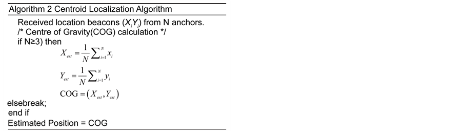
2.3. Centroid Localization Algorithm

This is a simple connectivity algorithm for the localization of objects. This algo-

rithm explores the inherent connectivity nature of WSN devices based on their proximity [12] . Sensor nodes within close proximity are likely to be connected baring extreme environmental conditions, physical obstruction or poor antenna orientation.

CLA is a coarse-grained algorithm that depends on reference nodes or anchors for location estimation. A free node locates its position using the intersection of the connectivity of the regions as defined by the radio range of each anchor. This is represented in the mathematical expression below:

(3)

where. In the above equation, is the estimated coordinate of the sensor or object to be localized, while and are the coordinates of the anchors participating in the localization. The pseudocode for CLA is as follows:

Various forms of modification to the original algorithm have been proposed. Foremost are some forms of weighting algorithms, otherwise referred to as Weighted Centroid Localization (WCL) algorithms [20] - [26] . All aimed at improving the position or location of the object to be localized. WCL algorithm estimates the location of unknown nodes by averaging the coordinates of the anchors within the vicinity of the unknown node. The anchors with the higher level of influence are weighted more heavily. However, a major drawback in the concept of WCL is the subjectivity of the weighting mechanism and the attendant overhead in determining the weighting factor for the anchors participating in the centroid localization.

There is a fundamental similarity between CLA and APIT algorithms, aside the fact that they are both proximity based algorithms. Both algorithms divide their area of anchor coverage as sensed by the free node into triangular coordinates. While CLA assumes equal weight to the received signal, APIT through a process, weighs the quality of the signal strength within the coverage area. APIT uses the best weighted triangles to estimate the most dominant region.

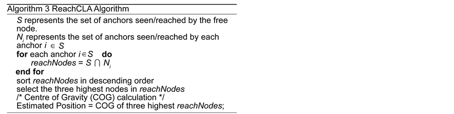
3. Reach Centroid Localization Algorithm

The relationship between transmitted and received signal is not symmetric. Two nodes transmitting and receiving signals between each other are likely not to receive each other’s signal at the same strength even if their power of transmission is the same. Many factors such as multipath effects account for this discrepancy. This situation or condition often leads to the erroneous localization of objects, particularly indoors. ReachCLA seeks to manage these conditions towards a more reliable estimation of the position of objects.

The algorithm establishes an authentication or feedback process between the free node and the anchors within its reach. In a global WSN environment, a free node is likely to receive signals from anchors within its immediate locality. These anchors are the ones within its reach and they are the ones that will participate in the localization process. ReachCLA has five main phases, they are summarized as follows:

・ The free node selects all the anchors that are within its reach.

・ The second phase is the feedback or handshake phase. This is to establish how the anchors read each other. This process is key as it allows the anchors establish their proximity to one another, and by so doing, they are able to reasonably ascertain the true position of the free node.

・ Selection of the anchors with the strongest reach. This is done as each selected anchor by the free node compare the anchors within their reach to other anchors selected by the free node.

・ Selection of the anchors with the three highest links or reach. Selection is from the group of anchors within the range of the free nodes, these are the anchors that have more anchors in common when matched with the anchors within the reach of the free node.

・ The COG of the three selected anchors is calculated, which will be the estimated location of the free node.

There are probable instances where an anchor within the reach of a free node will not be able to read the transmitted signal from the free node in a two way communication. However, because the anchor in case is able to communicate with other anchors that are within the reach of the free node, it therefore assures the likelihood or authenticates that the free node is within its own proximity. It is this authentication process that makes ReachCLA a unique and reliable algorithm for localization. An experimental testbed was set up to analyse the performance of ReachCLA alongside CLA and APIT algorithms.

4. Description of Testbed

Our experimental test-bed uses MICAz sensors manufactured by Crossbow Inc. The experiment was conducted indoors, using 5 rooms covering approximately 400 m² of space. A total of 17 MICAz nodes were used; one as a free node, another as the base station, while 15 served as anchors. The anchors were non- uniformly distributed. The nodes were connected through a MICAz that served as the base station to form a mesh network. The base station was docked on a programming board, which was connected to a laptop that was acting as the server. Figure 5 is the mapping of the deployment to the Euclidean coordinate

system. The region within the experimental area with reliable links between the anchors and free node was mapped as a 10 by 10 unit to the X and Y grid system to reflect a 2D layout of the nodes.

The base station was setup to act as the free node. The free node was static and RSS readings were set at a base value of −90 dBm. To ensure consistency, the tabulated signal readings were the collation of average RSS values and patterns over a period of 14 days. We ensured that environmental conditions were not modified or managed in any form. However, we ensured that all RSS readings were taken using the same MICAz nodes, while maintaining the anchors at a consistent coordinate throughout the experiment. Table 1 is a representation of the relationship between the anchors and the free node.

The free node has the anchors in column 1 within its reach, while column 4 shows the anchors that are visible to the anchor in column 1. For instance, the anchor with node ID 09 in column 1 is visible to the free node as shown in Table 2, while the anchors with node IDs 12, 14, 22, 23 and 21 in column 4 are all visible to anchor 09. The only relevance of column 2, which contains the RSS read

ings from the anchors as seen by the free node, is to select or determine the anchors that are within the range of the free node; in our case, the threshold RSS range was set at −90 dBm. It should be noted that these RSS values were not employed for any form of correlation with distance.

We simulated our proposed ReachCLA algorithm to estimate the position of the free node using Matlab. Figure 6 is the plot of the actual coordinates of the free node, which is 2, 4, while the estimated position is at the coordinate 1.67, 5.

Using the same data, we used the CLA to estimate the position of the free node. The comparative position of the object is as shown in Figure 7.

Figure 8 plots the APIT estimate of the location of the object, while Figure 9 presents the estimated positions of the ReachCLA, CLA and APIT.

5. Findings and Discussion

Figures 6-8 are the simulations of ReachCLA, CLA and APIT algorithms respectively. The simulations show the different estimated positions of the sensor node using each algorithm. Figure 9 presents the various estimated locations of the sensor node using ReachCLA, CLA and APIT on a single plot. The various plots indicate that the fundamental principle of ReachCLA is similar to that of CLA and APIT as they all embrace the formation of triangles within areas of discernible radio signal, and use the triangles to estimate the location of the intended object. However, the main distinction lies in the process of selecting the most likely triangle or triangles to be used for localization. This is where ReachCLA, as indicated in Table 3, outperforms both CLA and APIT.

In terms of timing, all the algorithms have similar convergence time, however, when it comes to the amount of memory used in processing the location of the free node, ReachCLA and CLA have similar memory usage, while APIT requires a lot of memory under a similar process. It should nevertheless be noted that in a region of high node density, the memory requirement for both CLA and particularly APIT will geometrically increase as the numbers of triangles that will be required for location estimation will geometrically increase.

The most significant factor here, as observed from our experiment, is the error margin. The error margin is the difference in distance between the true location of the object and the estimated location of the object (see Figure 9). Using Equation (4).

(4)

where d is the distance between the actual location and the estimated location of the sensor node; x, y and x_i, y_i are the actual and estimated coordinates of the sensor node respectively. ReachCLA outperforms both CLA and APIT in this regard. The error margins of both CLA and APIT are similar; they nonetheless, are thrice in magnitude to that of ReachCLA. The point here is that ReachCLA is better at managing radio signal vagaries due to changing environmental conditions in an enclosed environment. Hence, all the anchors participating or visible to the free-node are not of equal significance.

On the other hand, CLA and APIT assume equal weight of availability for all the anchors participating in the localization process. This is because CLA and APIT use RSS, which has an inherent susceptibility to environmental factors, as the key determinant factor for the selection of the anchors participating in the process. ReachCLA prioritizes the effects of the anchors that participate in the localization process based on the level of visibility of the anchors to one another and by so doing, mitigates the uncertainty surrounding the actual presence of an anchor based on the quality of the RSS for the anchor. Nonetheless, just as it is in APIT, we believe that performance of ReachCLA will degrade appreciably if the number of anchors falls below a certain threshold.

6. Conclusions

This paper is an attempt at contributing to the existing process of using WSN devices in the localization of objects in an enclosed environment. We proposed a proximity-based algorithm in this regard and compared its performance with similar algorithms such as, CLA and APIT. Based on the experiments conducted, it was observed that our algorithm outperformed both CLA and APIT in terms of resource consumption and accuracy.

Nevertheless, we realized that our proposed algorithm still needs to be subjected to more experimental rigours, as we have only used a simple and small test-bed to compare the performance of the algorithm. Our future work will be to implement the algorithm using a more robust and larger network to check for consistency in its performance. We will also need to validate the performance of the network using a dense and sparse WSN to determine both the limits of the accuracy of the algorithm and the minimum number of anchors required for localization.

Cite this paper

Ademuwagun, A. and Fabio, V. (2017) Reach Centroid Localization Algorithm. Wireless Sensor Network, 9, 87-101. https://doi.org/10.4236/wsn.2017.92005

References

- 1. Sharma, R. and Malhotra, S. (2015) Approximate Point in Triangulation (Apit) Based Localization Algorithm in Wireless Sensor Network. International Journal for Innovative Research in Science and Technology, 2, 39-42.
- 2. He, T., Huang, C., Blum, B.M., Stankovic, J.A. and Abdelzaher, T. (2003) Range-Free Localization Schemes for Large Scale Sensor Networks. Proceedings of the 9th Annual International Conference on Mobile Computing and Networking, San Diego, 14-19 September 2003, 81-95.
https://doi.org/10.1145/938985.938995 - 3. Dargie, W. and Poellabauer, C. (2010) Fundamentals of Wireless Sensor Networks: Theory and Practice. John Wiley & Sons, Hoboken.
https://doi.org/10.1002/9780470666388 - 4. Kumar, A., Kumar, V. and Kapoor, V. (2011) Range Free Localization Schemes for Wireless Sensor Networks. 10th WSEAS International Conference on Software Engineering, Cambridge, 22-24 February 2011, 101-106.
- 5. Karl, H. and Willig, A. (2007) Protocols and Architectures for Wireless Sensor Networks. John Wiley & Sons, Hoboken.
- 6. Kim, S.-Y. and Kwon, O.-H. (2005) Location Estimation Based on Edge Weights in Wireless Sensor Networks. The Journal of Korean Institute of Communications and Information Sciences, 30, 938-948.
- 7. Chong, C. and Kumar, S.P. (2003) Sensor Networks: Evolution, Opportunities, and Challenges. Proceedings of the IEEE, 91, 1247-1256.
https://doi.org/10.1109/JPROC.2003.814918 - 8. Li, X.-Y., Wan, P.-J. and Frieder, O. (2003) Coverage in Wireless Ad Hoc Sensor Networks. IEEE Transactions on Computers, 52, 753-763.
https://doi.org/10.1109/TC.2003.1204831 - 9. Lazos, L. and Poovendran, R. (2004) Serloc: Secure Range-Independent Localization for Wireless Sensor Networks. Proceedings of the 3rd ACM Workshop on Wireless Security, Philadelphia, 01 October 2004, 21-30.
https://doi.org/10.1145/1023646.1023650 - 10. Nagpal, R., Shrobe, H. and Bachrach, J. (2003) Organizing a Global Coordinate System from Local Information on an Ad Hoc Sensor Network. In: Zhao, F. and Guibas, L., Eds., Information Processing in Sensor Networks, Springer, Berlin, 333-348.
https://doi.org/10.1007/3-540-36978-3_22 - 11. Priyantha, N.B., Chakraborty, A. and Balakrishnan, H. (2000) The Cricket Location-Support System. Proceedings of the 6th Annual International Conference on Mobile Computing and Networking, Boston, 06-11 August 2000, 32-43.
- 12. Bulusu, N., Heidemann, J. and Estrin, D. (2000) Gps-Less Low-Cost Outdoor Localization for Very Small Devices. IEEE Personal Communications, 7, 28-34.
https://doi.org/10.1109/98.878533 - 13. Long, S., Wang, F., Duan, W. and Ren, F. (2004) Range-Free Self-Localization Mechanism and Algorithm for Wireless Sensor Networks. Computer Engineering and Applications, 23, 39.
- 14. He, T., Huang, C., Blum, B.M., Stankovic, J.A. and Abdelzaher, T.F. (2005) Range-Free Localization and Its Impact on Large Scale Sensor Networks. ACM Transactions on Embedded Computing Systems, 4, 877-906.
https://doi.org/10.1145/1113830.1113837 - 15. Rappaport, T.S. (1996) Wireless Communications: Principles and Practice. Vol. 2, Prentice Hall, Upper Saddle River.
- 16. Niculescu, D. and Nath, B. (2003) Dv Based Positioning in Ad Hoc Networks. Telecommunication Systems, 22, 267-280.
https://doi.org/10.1023/A:1023403323460 - 17. Keshtgary, M., Fasihy, M. and Ronaghi, Z. (2011) Performance Evaluation of Hop-Based Range-Free Localization Methods in Wireless Sensor Networks. ISRN Communications and Networking, 2011, Article ID: 485486.
https://doi.org/10.5402/2011/485486 - 18. Kleinrock, L. and Silvester, J. (1978) Optimum Transmission Radii for Packet Radio Networks or Why Six Is a Magic Number. Proceedings of the IEEE National Telecommunications Conference, 4, 1-4.
- 19. Wang, J. and Jin, H. (2009) Improvement on Apit Localization Algorithms for Wireless Sensor Networks. International Conference on Networks Security, Wireless Communications and Trusted Computing, 1, 719-723.
https://doi.org/10.1109/nswctc.2009.370 - 20. Zhao, J., Zhao, Q., Li, Z. and Liu, Y. (2013) An Improved Weighted Centroid Localization Algorithm Based on Difference of Estimated Distances for Wireless Sensor Networks. Telecommunication Systems, 53, 25-31.
https://doi.org/10.1007/s11235-013-9673-6 - 21. Dong, Q. and Xu, X. (2014) A Novel Weighted Centroid Localization Algorithm Based on RSSI for an Outdoor Environment. Journal of Communications, 9, 279-285.
https://doi.org/10.12720/jcm.9.3.279-285 - 22. Zhu, Z., He, X., Zhang, X., Zhao, S. and Xia, Y. (2014) The Quadrilateral and Improved Weighted Centroid Localization Algorithm Based on RSSI. Journal of Hangzhou Dianzi University, 1, 004.
- 23. Ding, E.J., Qiao, X., Chang, F. and Qiao, L. (2013) Improvement of Weighted Centroid Localization Algorithm for WSNS Based on RSSI. Transducer and Microsystem Technologies, 32, 53-56.
- 24. Zhang, B., Ji, M. and Shan, L. (2012) A Weighted Centroid Localization Algorithm Based on Dv-Hop for Wireless Sensor Network. 8th International Conference on Wireless Communications, Networking and Mobile Computing, Barcelona, 21-23 September 2012, 1-5.
https://doi.org/10.1109/wicom.2012.6478383 - 25. Shi, H. (2012) A New Weighted Centroid Localization Algorithm Based on RSSI. International Conference on Information and Automation, Shenyang, 6-8 June 2012, 137-141.
https://doi.org/10.1109/icinfa.2012.6246797 - 26. Wang, Z.-M. and Zheng, Y. (2014) The Study of the Weighted Centroid Localization Algorithm Based on RSSI. International Conference on Wireless Communication and Sensor Network, Wuhan, 13-14 December 2014, 276-279.