Engineering
Vol.4 No.12(2012), Article ID:25740,4 pages DOI:10.4236/eng.2012.412107
Finite Element Analysis with Paraxial & Viscous Boundary Conditions for Elastic Wave Propagation
Structural Engineering Research Division, Korea Institute of Construction Technology, Ilsan, South Korea
Email: lagoon@kict.re.kr
Received October 8, 2012; revised November 9, 2012; accepted November 19, 2012
Keywords: Paraxial Boundary; Local Boundary; Penalty Functional; Viscous Boundary
ABSTRACT
In this study, two studies are performed. One is to apply paraxial boundary conditions which are local boundary conditions based on paraxial approximations of the one-way wave equations to finite element analysis. To do this, a penalty functional is proposed and the existence and uniqueness of the extremum of the proposed functional is demonstrated. The other is to improve the capacity of viscous boundary conditions using dashpots. To do this, customary viscous boundary conditions are modified to maximize the efficiency according to angles of incidence and materials. For the numerical analysis of elasticity with paraxial boundary conditions and the modified viscous boundary conditions, the coding of the finite element models is implemented, and the efficiency of those boundary conditions is investigated.
1. Introduction
In many dynamic problems, the analysts are confronted with the problem of wave propagation in infinite or semiinfinite media. The complex geometry or/and non-homogeneity disturb or prohibit to find the closed-form solutions to those problems. In this reason various numerical techniques are needed. But since such discrete models used are necessarily finite in size, echoes would develop at the artificial boundaries if no appropriate action was taken. Absorbing boundaries are mathematical artifacts used to prevent wave reflections at the boundaries of discrete models for infinite media under dynamic loads. A number of these boundaries have been proposed in the past three decades and used with various degrees of success. The collection of absorbing boundaries can be grouped into two broad classes: nonlocal and local absorbing boundaries. Nonlocal boundaries are exact, robust, accurate, and stable, but some of those are properly defined only in the frequency domain, and cannot be used for problems involving material nonlinear effects. And for some of those the exact condition is not available or is too complicated to be practical. For these reasons, a number of local absorbing boundaries have been proposed. Local absorbing boundaries may be good energy absorbers, but they are not perfect ones, therefore, a residual echo may be present in the solution. However, the accuracy of some classes of the local absorbing boundaries can be increased by taking higher order approximations for boundary conditions. But the various sequence of such boundary conditions make the absorbing boundary conditions have complex mathematical forms with partial derivatives, and thus this complicates the application of such local absorbing boundary conditions to finite element analysis. Paraxial boundary conditions are such kinds of local boundary conditions, which are based on paraxial approximations of the one-way wave equations, and thus the application of those to finite element analysis is difficult. In this study, to do this, a penalty functional is newly proposed and the existence and uniqueness of the extremum of the proposed functional is demonstrated. The penalty functional proposed in this study enables to derive the functional including not only the total potential energy but also paraxial boundary conditions in elastic media and thus to analyze the elasticity problems with the paraxial boundary conditions. Consequently, it may be expected that the proposed approach can be applied to any local boundary conditions based on approximations of the one-way wave equations. Viscous boundary conditions which are also some kinds of local boundary conditions are most convenient to apply to finite element analysis, but it is known that the capacity is not good. In this study the study on improving the capacity of viscous boundary conditions is implemented. Using the concept of energy ratio between the reflected waves and the incident wave, the efficiency of customary viscous boundary conditions can be improved for an arbitrary angle of incidence and materials. Finally, for the numerical analysis of elasticity with paraxial boundary conditions and the modified viscous boundary conditions, the coding of the finite element models is implemented, and the efficiency of those boundary conditions is investigated.
2. Paraxial and Viscous Boundary Conditions
2.1. Paraxial Boundary Conditions
Paraxial boundary conditions are based on the paraxial approximations of the one-way wave equations, which were developed for scalar wave equation [1-3] and for the elastic wave [4]. The absorbing boundary conditions should be chosen such that its dispersion relation is a good approximation of the interior dispersion relation for outgoing waves, and the boundary conditions together with the differential equation should form a well posed problem. The better the boundary conditions describe outgoing waves the smaller will be the reflection [5].
Figure 1 schematically shows the dispersion relation for a plane wave and Equation (1) is its mathematical form, where ,
,  are xand y-directional spatial wave lengths, and
  and
and  are xand y-directional wave numbers respectively.
Using Equation (1), the first and the second down-going paraxial boundary conditions, Equations (2) and (3) can be derived [6].
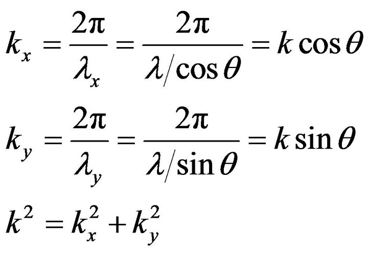 (1)
(1)
 (2)
(2)
 (3)
(3)

Figure 1. Dispersion relation for a plane wave.
2.2. Viscous Boundary Conditions
Figure 2 shows the basic idea of a viscous boundary for plane strain. The energy arriving at the boundary in Figure 2 will be absorbed if tractions, Equations (4)-(5) are applied to the boundary which are equal in magnitude and opposite in direction to the stresses caused by the incident wave.
 (4)
(4)
 (5)
(5)
In Equations (4) and (5) the parameters, a and b, vary according to not only the incident angles but also the material properties of the medium. The choice of a = b = 1 which is called “the standard viscous boundary” was given by Lysmer and Kuhlemeyer (1969) [7] for the whole range of incident angles. The absorption by viscous boundary conditions cannot be made perfect over the whole range of incident angles and/or for all the material properties of medium, but can be made maximum. Hence, the parameters a and b in Equations (4) and (5) can be chosen to maximize the efficiency of the viscous boundary conditions for an arbitrary angle of incidence and material through which waves propagate. A good measure for the ability of the viscous boundary to absorb impinging elastic waves is the energy ratio defined as the ratio between the transmitted energy of the reflected waves and the transmitted energy of the incident wave. This ratio can be computed from the wave amplitudes ratios by considering the energy flow to and from a unit area of the boundary. The situations for an incident compressional and shear waves are shown in Figure 3.
The absorption ratio (AR) of the viscous boundary according to the incident angles can be defined such that
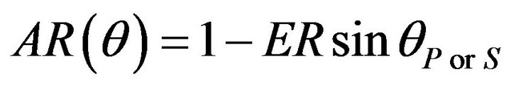 (6)
(6)
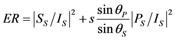
where energy ratio (ER) is defined as follows, for incident compressional wave
 (7)
(7)
and for incident shear wave Case 1: Incident angle θ greater than the critical angle 

Figure 2. Schematic representation of a viscous boundary.

Figure 3. Incident compressional (P) and shear (S) waves.
 (8a)
(8a)
Case 2: Incident angle  less than the critical angle
 (8b)
(8b)
In Equation (7) ,
,  , and
, and  are the complex amplitudes of the incident compressional, the reflected compressional, and the reflected shear waves and s is the ratio of the shear wave velocity to the compressional wave velocity. In Equations (8a) and (8b)
 ,
,  , and
, and  are the complex amplitudes of the incident shear, the reflected compressional, and the reflected shear waves.
Equation (6) can be used to maximize the efficiency of viscous boundary conditions (Equations (4) and (5)), and varying the parameters a and b in Equations (4) and (5) to maximize Equation (6) according to incident angles and Poisson’s ratios gives Table 1 for incident compressional wave and Table 2 for incident shear wave.
2.3. Comparison of Paraxial to Viscous Boundary Conditions
Figures 4-7 show the amplitude ratios between the incident, the reflected compressional, and the reflected shear waves, where “This study”, “Paraxial 1”, “Paraxial 2”, “Lysmer (1969)”, and “White (1977)” denote the results of the viscous boundary conditions modified in this study, the paraxial boundary conditions (Equation (2)), the paraxial boundary conditions (Equation (3)), Lysmer-Kuhlemeyer (1969) [7]’s boundary conditions, and White et al. (1977) [8]’s boundary conditions, respectively.

Table 1. Values of a and b for P-wave incidence.

Table 2. Values of a and b S-wave incidence.

Figure 4. Amplitude ratio of the reflected P-wave to the incident P-wave.
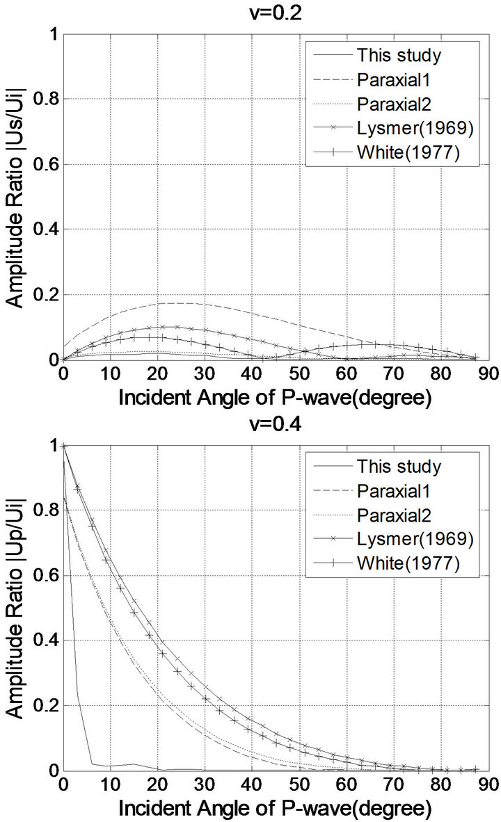
Figure 5. Amplitude ratio of the reflected S-wave to the incident P-wave.

Figure 6. Amplitude ratio of the reflected P-wave to the incident S-wave.
In Figures 4-7 the compressional and shear reflections are shown for incident P and S wave. Here, it can be seen that all of the boundaries but the viscous boundary modified in this study are nearly equal in their reflection amplitudes. Near to perfect absorption is attained for those incident waves which are almost normal to the boundary. Conversely, total reflection occurs for the waves which impinge at 0˚ angles. All the boundaries are almost as effective for lower Poisson’s ratios as they are for higher ones. Figures 4-7 show that the modified viscous boundary clearly outperforms its competitors.
3. Finite Element Analysis of Paraxial and Viscous Boundary Conditions
3.1. Variational Formulation of Paraxial Bounary Conditions
The functional, Equation (9), makes the finite element analysis of the paraxial boundary conditions easy because the governing equations which are derived from the proposed penalty functional include the paraxial boundary conditions in itself, and thus the development of any special numerical integration schemes and interpolation functions are not required.
 (9)
(9)
where K,  ,
, ![]() ,
,  ,
,  , and
, and  are the kinetic energy, the total potential energy, the variational operator, penalty functions, the paraxial boundary conditions, and displacements respectively.
The first term in Equation (9) (i.e., the functional including K and ) has the extremum and it is unique. Hence, if the extremum for the second term in Equation (9) exists and is unique, the extremum for the total functional, Equation (9), will exist and be unique. The existence and uniqueness of the second term in Equation (9) was already proved by Kim and Lee (2008) [6].

Figure 7. Amplitude ratio of the reflected S-wave to the incident S-wave.
3.2. Finite Element Formulation of Paraxial Boundary Conditions
The vector forms, Equations (10) and (11), of the finite element model for the paraxial boundary conditions can be obtained by substituting Equations (2) and (3) into Equation (9) such that
 (10)
(10)
 (11)
(11)
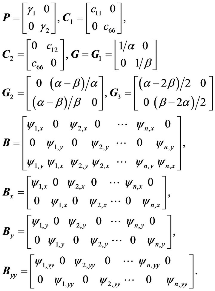
where ψ, C, and f are the matrices related to interpolation functions, elastic stiffnesses, and body forces respectively, and the rest matrices in Equations (10) and (11) are [6]
3.3. Finite Element Formulation of Viscous Boundary Conditions
The viscous boundary conditions, Equations (4) and (5), correspond to a situation in which the convex boundary is supported on infinitesimal dashpots oriented normal and tangential to the boundary. Hence the variational formulation can be used to apply the viscous boundary to a finite element model.
![]()
(12)
where

3.4. Numerical Example
To investigate the efficiency of the paraxial and the modified viscous boundary conditions, the displacements between Models (a) and (b) in Figure 8 are compared each other. Model (a), of which boundaries are fixed and which is extensive enough to prevent the boundary reflections reaching the interior zone, is horizontally about four times and vertically about two times larger than Model (b) including the paraxial and viscous boundary conditions at the boundaries. In all the models, the elastic regions are discretized with nine-noded elements which employ quadratic isoparametric interpolation functions, where 10,000 elements are used in Model (a) and 676 elements in Model (b). The used elastic moduli, Young’s modulus E and Poisson ratio v, and mass density ρ are presented in Table 3.
Figure 9 reports the horizontal and vertical displacements recorded at A and C in Models (a) and (b), where “Lysmer”, “White”, and “This study” indicate the viscous boundaries proposed by Lysmer-Kuhlemeyer (1969) [7], White et al. (1977) [8], and this study respectively. And “Paraxial 1” denotes the paraxial boundary conditions, Equation (2). “Reference” and “free” are respectively referred to the solutions in Model (a) and Model (b) where traction free condition is applied.

Figure 8. Numerical models.

Table 3. Elastic moduli and mass density.


Figure 9. Horizontal and vertical displacements at A and C in Models (a) and (b).
Wave reflections caused by a free boundary are clearly seen in Figure 9, while the viscous and paraxial boundaries largely succeed in eliminating these reflections. Aslo, since the waves induced by a dynamic load in Figure 8 are absorbed firstly at the boundary along which the paraxial and viscous boundaries are applied and the residual echoes propagate into the interior region. Figure 9 also shows that, in the case of the vertical displacements, the paraxial boundary is slightly more accurate, and demonstrates how well the finite element model, Equation (10), induced from the proposed functional, Equation (9), simulates the infinite domain.
4. Conclusions
In this study, studies on applying the paraxial boundary conditions to finite element analysis and improving the capacity of viscous boundary conditions were implemented, and the following results could be obtained:
1) Using the penalty functional modified in this study, the functional for elasticity with the paraxial boundary conditions can be obtained, and this makes the finite element formulation of the paraxial boundary conditions possible.
2) Moreover, since, solving the finite element models derived from the obtained functional, any special numerical scheme and interpolation function are not required, this method can be applied to any other local absorbing boundary conditions.
3) Using the concept of energy ratio between the transmitted energy of the reflected waves and the transmitted energy of the incident wave per unit of time through a unit area of the wave front of compressional and shear waves, the efficiency of the viscous boundary conditions for the compressional and the shear waves can be improved for an arbitrary angle of incidence and materials.
REFERENCES
- J. F. Claerbout, “Coarse Grid Calculations of Waves in Inhomogeneous Media with Application to Delineation of Complicated Seismic Structure,” Geophysics, Vol. 35, No. 3, 1970, pp. 407-418. doi:10.1190/1.1440103
- J. F. Claerbout, “Fundamentals of Geophysical Data Processing,” McGraw-Hill, New York, 1976.
- J. F. Claerbout and A. G. Johnson, “Extrapolation of Time Dependent Waveforms along Their Path of Propagation,” Geophysical Journal of the Royal Astron Society, Vol. 26, No. 1-4, 1971, pp. 285-293. doi:10.1111/j.1365-246X.1971.tb03402.x
- R. Clayton and B. Engquist, “Absorbing Boundary Conditions for Acoustic and Elastic Wave Equations,” Bulletin of the Seismological Society of America, Vol. 67, No. 6, 19977, pp. 1529-1540.
- B. Engquist and A. Majda, “Absorbing Boundary Conditions for the Numerical Simulation of Waves,” Mathematics of Computation, Vol. 31, No. 139, 1977, pp. 629-651. doi:10.1090/S0025-5718-1977-0436612-4
- H. S. Kim and J. S. Lee, “Finite Element Analysis with Paraxial Boundary Conditions for Elastic Wave Propagation,” Proceedings of 15 International Congress on Sound and Vibration, Daejeon, 6-10 June 2008.
- J. Lysmer and R. L. Kuhlemeyer, “Finite Dynamic Model for Infinite Media,” Journal of the Engineering Mechanics Division, Vol. 95, No. EM4, 1969, pp. 859-877.
- W. White, S. Valliappan and I. K. Lee, “Unified Boundary for Finite Dynamic Models,” Journal of the Engineering Mechanics Division, Vol. 103, No. EM5, 1977, pp. 949- 964.