Circuits and Systems
Vol.07 No.04(2016), Article ID:65478,13 pages
10.4236/cs.2016.74016
A Novel Flower Pollination Algorithm to Solve Load Frequency Control for a Hydro-Thermal Deregulated Power System
D. Lakshmi1, A. Peer Fathima2, Ranganath Muthu3
1Department of Electrical and Electronics Engineering, Sree Sastha Institute of Engineering and Technology, Chennai, India
2School of Electrical Engineering, Vellore Institute of Technology, Chennai, India
3Department of Electrical and Electronics Engineering, SSN College of Engineering, Kalavakam, Chennai, India

Copyright © 2016 by authors and Scientific Research Publishing Inc.
This work is licensed under the Creative Commons Attribution International License (CC BY).
http://creativecommons.org/licenses/by/4.0/


Received 21 March 2016; accepted 10 April 2016; published 13 April 2016
ABSTRACT
Load frequency control plays a vital role in power system operation and control. LFC regulates the frequency of larger interconnected power systems and keeps the net interchange of power between the pool members at predetermined values for the corresponding changes in load demand. In this paper, the two-area, hydrothermal deregulated power system is considered with Redox Flow Batteries (RFB) in both the areas. RFB is an energy storage device, which converts electrical energy into chemical energy, that is used to meet the sudden requirement of real power load and hence very effective in reducing the peak shoots. With conventional proportional-integral (PI) controller, it is difficult to get the optimum solution. Hence, intelligent techniques are used to tune the PI controller of the LFC to improve the dynamic response. In the family of intelligent techniques, a recent nature inspired algorithm called the Flower Pollination Algorithm (FPA) gives the global minima solution. The optimal value of the controller is determined by minimizing the ISE. The results show that the proposed FPA tuned PI controller improves the dynamic response of the deregulated system faster than the PI controller for different cases. The simulation is implemented in MATLAB environment.
Keywords:
Load Frequency Control, Redox Flow Battery, Proportional Integral Controller, Flower Pollination Algorithm

1. Introduction
The complexity of power system is highly increasing due to the rapid increase in load. Operation and control of power system become an important task for secured and reliable operation. The objective of the LFC is to maintain the system frequency and tie line power flow constant for a transient change in load [1] . The standards related to LFC are given by the IEEE Committee report [2] . In the literature, hydro and thermal systems have been handled by LFC [3] .
With the development in the power industry, the power system is in transition for restructuring and deregulation. Many researchers analyzed the problem of LFC in a deregulated environment for the past nine decades [4] [5] . Donde et al. [6] discussed the concept of DPM (Disco Participation Matrix) and Area control error participation factor (Apf) for a bilateral structure in the deregulated environment.
Many control strategies were employed in the past nine decades, to reduce the oscillations of change in frequency and tie-line power flow. Proportional Integral (PI) controller is mostly used as a controller in LFC because of ease of operation [7] [8] . In order to make the operation of power system more reliable, energy storage devices are included in deregulated power system.
Several energy storage systems were available such Superconducting Energy storage system, batteries, etc. Tetsuo Sasaki et al. discussed that rechargeable batteries are not aged by frequent charging and discharging and have better response during overload when compared to other energy storage systems [9] . Chidambaram et al. have explained the use of RFB in LFC to improve the dynamic response of the deregulated power system along with Interline Power flow controller (IPFC) in the tie line [10] .
In this work, a two-area deregulated power system is considered in which area1 has two DISCOs, two non- reheat thermal units as GENCO1 and GENCO2. Similarly, area2 has two DISCOs, two hydro units as GENCO3 and GENCO4. Proportional Integral (PI) controller is used and the gain values were tuned by using Ziegler-Ni- chols and Flower Pollination algorithm. The performance of the controller was analyzed by using performance index. Further, an Energy storage device Redox Flow Batteries (RFB) was used to improve the LFC performance. The RFB stores energy and dissipates at a faster rate whenever required.
In this paper, Section 2 explains the block diagram model of two-area hydrothermal deregulated power system and Redox Flow battery principle of working. The overall transfer function model is explained in Section 3. Section 4 explains the tuning of the PI controller by Ziegler-Nichols and FPA. The simulation of the hydrothermal deregulated power system for different cases with PI controller and FPA tuned PI controller followed by a discussion is given in Section 5. From the simulation results and discussion, the conclusion is made in Section 6.
2. Hydrothermal Deregulated Power System
The power system model consists of two control areas connected by a tie line as shown in Figure 1. Area1 consists of two DISCO1, DISCO2, two non-reheat thermal units GENCO1 and GENCO2. Similarly, area2 consists of two DISCO3, DISCO4, two hydro units as GENCO3 and GENCO4. The concept of DISCO Participation

Figure 1. Schematic diagram of the two area deregulated power system.
Matrix (DPM), to visualize the contracts between GENCOs and DISCOs was introduced [5] . DPM is a matrix in which number of rows is equal to the number of GENCOs and the number of columns is equal to the number DISCOs in the system. The sum of all entries in a column of DPM must be Unity.
In the proposed deregulated system as shown in Figure 1, there are two non-reheat thermal units, two hydro units as GENCOs and two DISCOs in area1 and area2. The corresponding DPM is shown as in Equation (1) in which the entities are called as “cpf” represents contract participation factor i.e. pu Mw load of corresponding DISCO.
 with
with  (1)
(1)
where 
Principle of Operation of Redox Flow Batteries
Batteries are devices that store chemical energy and generate electricity by a reduction-oxidation (redox) reaction: i.e. a transformation of matter by electron transfer. The redox (reduction-oxidation) cell is a reversible fuel cell in which all electrochemical components are dissolved in the electrolyte. Redox flow batteries are rechargeable [12] . Some types of Redox Flow Batteries are the Vanadium redox flow battery, polysulfide bromide battery and uranium redox flow battery. The vanadium redox flow battery is used in the work under consideration.
A vanadium RFB consists of an assembly of power cells in which the two electrolytes are separated by a proton exchange membrane. Figure 2 shows the working of the Redox Flow Battery. Both the electrolytes are vanadium based, the electrolyte in the positive half-cells contain  and
and  ions, the electrolyte in the negative half-cells,
  and
and  ions. The electrolytes may be prepared by any of several processes, including electrolytically dissolving vanadium pent oxide (V2O5) in sulfuric acid (H2SO4). The solution remains strongly acidic in use.
The following equations represent the working of the vanadium redox flow


 (2)
(2)

Figure 2. Working principle of redox flow battery.
where water (H2O) and protons (H+) are required in the cathodic reaction to maintain the charge balance. The advantages of RFB over the other energy storage systems are easy maintenance, load following, storage for long time period and fast response.
RFB, placed in both the areas to damp out oscillations i.e. improves the dynamic response of change in frequency and tie line power flow. RFB is placed in the area will be charged from the power from the units under balance condition. When the load demand increases the energy stored in the battery is released to the system. As the control mechanism brings the system to its new equilibrium condition, the battery charges it to its full value. Similarly, when the load decreases, the battery gets charged absorbing the excess power in the system. The absorbed excess power is released back after the system returns to its steady state.
3. Transfer Function Model of Deregulated Power System
Area 1 consists of two GENCOs, which have two identical non-reheat thermal units, and two DISCOs; Area2 has two GENCOs, which have two identical hydro units, and two DISCOs. Figure 3 shows the transfer function model of system, in which R1, R2, R3 and R4 are the governor regulation parameters of thermal units and hydro units for area1 and area2 in Hz /pu.MW respectively.
Area1 consists of two speed governing system, two non-reheat turbines and area2 has two mechanical hydro governor and hydro turbine. In order to simplify the frequency domain analysis, the transfer function is used to represent the components of the area.
3.1. Transfer Function of Thermal Units
The transfer function of speed governor of area1 is given by Equation (3)
 (3)
(3)
where KGj is the gain of the jth governor and TGj is the time constant of the jth governor.
The non-reheat turbine model is given by Equation (4)
 (4)
(4)
where, KTj is the gain of the jth non-reheat turbine and TTj is the time constant of the jth non-reheat turbine.
3.2. Transfer Function of Hydro Units
In hydro units, water is the main source for producing mechanical energy, which is the input to the turbine. Function of speed governor of hydro unit is similar to that of steam governor. In this work, the low head hydro unit is considered [11] . The transfer function of hydro governor is given by Equations (5) and (6).
 (5)
(5)
where, KHj is the gain of the jth hydro governor and THj is the time constant of the jth hydro governor.
 (6)
(6)
where, TRj is the reset time of the jth hydraulic amplifier and T2j is the time constant of the jth hydraulic amplifier.
Water is used as an input for the turbine and is connected to hydro governor. Transfer function of hydro turbine is given by Equation (7)
 (7)
(7)
where Twj is the time constant of the jth hydro turbine.
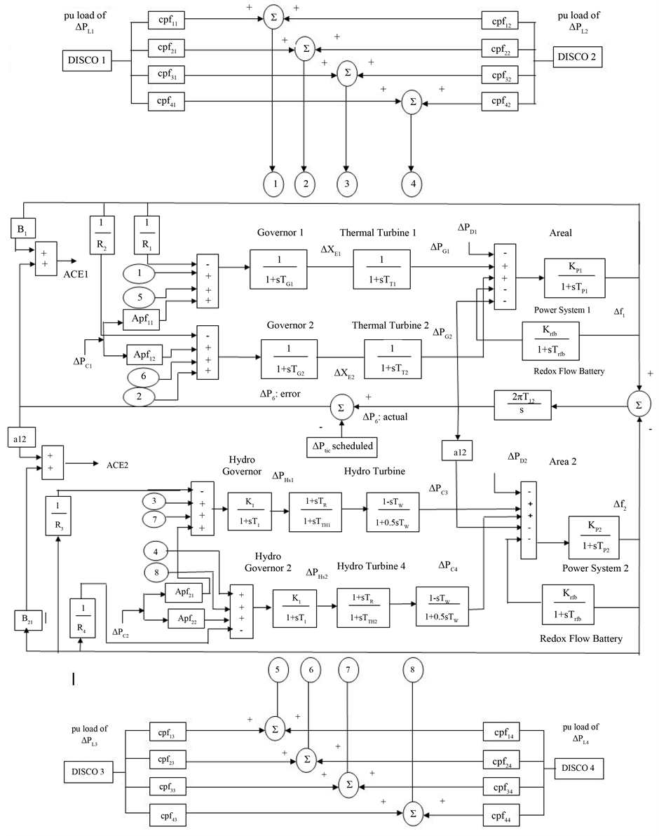
Figure 3. Transfer Function of Hydro thermal deregulated power system.
3.3. Transfer Function of Overall Power System
The model of the power system is given by Equation (8)
 (8)
(8)
where, KP is the gain of the ith area power system and TP is the time constant of the ith area power system.
The values of KP and TP are given by  and
and  where, H is per unit inertia constant, f is
system frequency and Di is expressed as percent change in load by percent change in frequency.
The scheduled steady state tie line power flow from area1 to area2 is the difference between the demand of DISCOs in the area2 from GENCOs in the area1 and the demand of DISCOs in area1 from the GENCOs in area2, which is given in Equation (9),
 (9)
(9)
The tie line power flow from area1 to area2 is the product of the tie line coefficient and the difference between the change in frequency in area 1 and the change in frequency in area2, as given by Equation (10),
 (10)
(10)
Equation (11) gives the error in the tie line power flow from area1 to area2, which is the difference between the actual and scheduled value of the tie line power.
 (11)
(11)
Equation (12) gives the error in tie line power flow from area2 to area1 is given.
 (12)
(12)
As both the areas are assumed to be identical, a12 = −1.
Equation (13) gives the Area Control Error (ACE) of area1, which is the summation of the bias factor with the deviation of the frequency and the change in tie-line power flows. Similarly, Equation (14) gives the ACE of area2.
 (13)
(13)
 (14)
(14)
As there are more than one GENCOs in each area, the Area Control Error (ACE) signal has to be given in proportion to their participation in LFC. The coefficient that distributes the ACE to all GENCOs is called as “ACE participation factor” (Apf). The summation of Apf should be always unity for each area. Hence, the ACE Participation factors for area 1 are Apf11, Apf12. Similarly, for the area2 are Apf21, Apf22.
3.4. Modelling of RFB in LFC
Redox Flow Battery (RFB) is connected to the power system of both areas, in which the input given is the change in frequency (real power) of that area and output will be as per the load requirement and either charges or discharges the power. As RFB has fast response, hunting due to delay in response does not occur [12] . Because of this reason, ACE is fed directly as a command signal LFC to control the output of RFB. Transfer function model of RFB is as shown in Figure 5 and the change in power (ΔPrfb) is given Equation (15)
 (15)
(15)
where Krfb is the gain of a RFB and Trfb is the time constant of RFB in seconds.
4. Controllers for LFC
The performance of the system poor and even possibly unstable, if the controllers are not tuned properly. The conventional PI controller is tuned by Ziegler-Nichols and FPA methods.
4.1. Conventional PI Controller
Proportional control mode will be good when the rate of change of error is high and this mode improves the transient performance. The Integral control mode is efficient when the error is low and this mode improves the steady state. The derivative control mode increases the noise and makes the system less stable because of its high sensitivity even though it has the advantage of reducing the overshoot [7] [8] . As the load is subjected to change, the derivative mode makes the system unstable.
In this work, the Proportional Integral controller because of its simplicity and flexibility. The mathematical model of PI controller is given in Equation (16).
 (16)
(16)
where KP is the P controller gain and KI is I controller gain and UPI is the controlled output of the PI controller and ACE is the Area Control Error of the concerned area.
4.2. Tuning of PI Using Artificial Optimization Algorithm
In designing the optimization based PI controller, the objective function may be defined based on the desired specifications and proper parameter settings to ensure that the system stable. Performance Indices that are usually used in design are Integral Time Absolute Error (ITAE), Integral Squared Error (ISE), Integral Time Squared Error (ITSE) and Integral Absolute Error (IAE). In this paper, the ISE is used as the objective function to optimize the parameters of the PI controller because this index will reduce larger errors quickly resulting in the fast response to the system.
Equation (17) gives the performance index used to optimize (minimization of the error).
 (17)
(17)
where Δf1 and Δf2 are the change in frequency of area1 and area2 and ΔPtie1,2 is the change in tieline power flow.
4.2.1. Flower Pollination Algorithm
One of nature inspired population based algorithm is Flower Pollination Algorithm (FPA) proposed by Xin-she Yang (2012). The primary aim of this FPA is to produce the optimal reproduction of plant species by surviving the fittest of the flowering plants.
In this world, there are a million types of flowering plants in nature, 80% of them were flowering species. The main purpose of a flower is ultimately reproduction via pollination. Transfer of pollens from one flower to another flower on the same plant (self-Pollination-Abiotic) or another plant (Cross Pollination-Biotic). This transformation may occur by pollinators such as wind, birds, insects, bats and other animals. FPA has better performance when compare to others in terms of accuracy, and convergence speed [13] - [15] .
The following four rules were employed to explain concept of flower pollination
1) Cross Pollination and Biotic were considered as Global Pollination and pollinators movement is considered which follows the Levy flight movement.
2) Local Pollination takes place in Abiotic and self-Pollination.
3) Pollinators like birds, insects may develop flower constancy, which is equivalent to the reproduction probability and will be proportional to the similarity of two flowers involved.
4) Switching from local to global pollination or vice versa can be controlled by the probability p ∈ [0, 1].
In global pollination, pollinators like birds, wind, insects carry out flower pollen and they travel over a long distance. This global pollination (i.e. rule 1 and 3) can be written as in Equation (18)
 (18)
(18)
where xik is the pollen i at iteration k, g* is the current best solution among the solutions for the current iteration. Here γ is the scaling factor used to control the step size. L(λ) is the step size parameter, in specific the Levy-flights-movement which shows the strength of the pollination.
As the pollinators travel over a long distance with different distance movements, levy flight is used to show the travelling characteristic which is shown in Equation (19). Assume L > 0 forms the Levy distribution.
 (19)
(19)
where Г(λ) is the standard gamma function and Levy distribution will be valid for longer steps S > 0. Rule 2 and 3 were for local pollination can be shown in Equation (20) as follows
 (20)
(20)
where ε is a local random lie from 0 to 1. Figure 4 shows the flowchart of FPA for tuning the gain values of PI.

Figure 4. Flowchart of FPA for tuning the gains of PI controller.
4.2.2. Design of FPA Based PI Controller
The objective function is to minimize the objective shown in Equation (17). Number of flowers is 20 and the maximum number of iterations is 100.
Step 1: Initialize the population of flowers (control variables P and I of each area)
Step 2: Calculate the fitness function of each flower (i.e. Min ISE) and select the global flower from the population
Step3: For each flower generate a random number, if the random number less than switch probability go to step 5
Step 4: Implement global pollination and go to step 6
Step 5: select a flower randomly for local pollination, then go to step
Step 6: pollinate a flower with global flower by using  where xi is the values of KP and KI.
Step 7: up to N number of flowers do step 2 to 6
Step 8: go to step 3 to 6 till the maximum iterations is reached, get the global flower as the best fitness value index (optimal values of KP and KI of the controller).
5. Case Studies and Simulation Results
For the transfer function diagram shown in Figure 2, simulation was carried out on MATLAB-Simulink [16] . Both the areas are assumed identical. Non-reheat turbine model is considered and the governor-turbine units of GENCO1 and GENCO2 were assumed to be identical and hydro turbine model of GENCO3 and GENCO4 were assumed to be identical. The Redox Flow Battery is added in both the areas and the values used are given in Appendix. Based on the transaction made between them, there are three types of transaction. If a DISCO has the contract with the GENCO of the same area is called as Pool-Co (Charged) transaction and if a DISCO has a contract with a GENCO of another area is called as bilateral transactions. Two different transactions were considered as follows.
5.1. Case 1
Pool-co transaction i.e GENCO in each are participate equally in LFC. Area Control Error (ACE) participator factor (Apf’s) is as follows:
 ,
,  ,
,  ,
,  and
and 
DISCOs have contracted with each GENCO. Assume load change occurs in area1 alone, i.e. 0.1 (pu MW) load change in DISCO1 and DISCO2. DISCO3 and DISCO4 does not demand power from any other GENCOs, then corresponding “cpfs” is zero. The DPM for the above case is as follows

In addition, the demand of DISCOs in (pu MW) is as follows: ΔPL1 = 0.1, ΔPL2 = 0.1, ΔPL3 = 0, ΔPL4 = 0. Since the uncontracted load is taken to be zero ΔPUC1 = 0, ΔPUC2 = 0. The scheduled tie-line power flow over the tie-line is zero, i.e. under steady state condition the generation of GENCOs must match the demand of the DISCOs in contract with it. The generated power (or) contracted power supplied by the GENCO is given as
 (21)
(21)
By using equation 21, ΔPg1 = 0.1 (pu∙Mw), ΔPg2 = 0.1(pu∙Mw), ΔPg3 = 0 (pu∙Mw) and ΔPg4 = 0 (pu∙Mw).
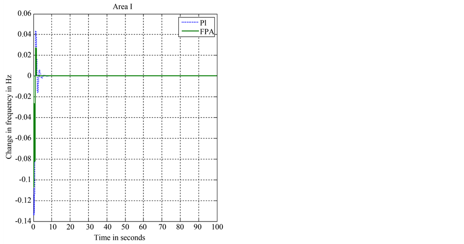
Figures 5(a)-(c) show the comparison of PI and FPA tuned PI controller for dynamic response of change in frequency (Hz) for each area and the tie line power flow (pu∙MW) between them which settles at 0.00 (pu∙MW). From Figures 5(a)-(c) it can be inferred that FPA tuned gain values of PI controller gives better results in terms of settling time, overshoot and undershoot.
 (a)
(a)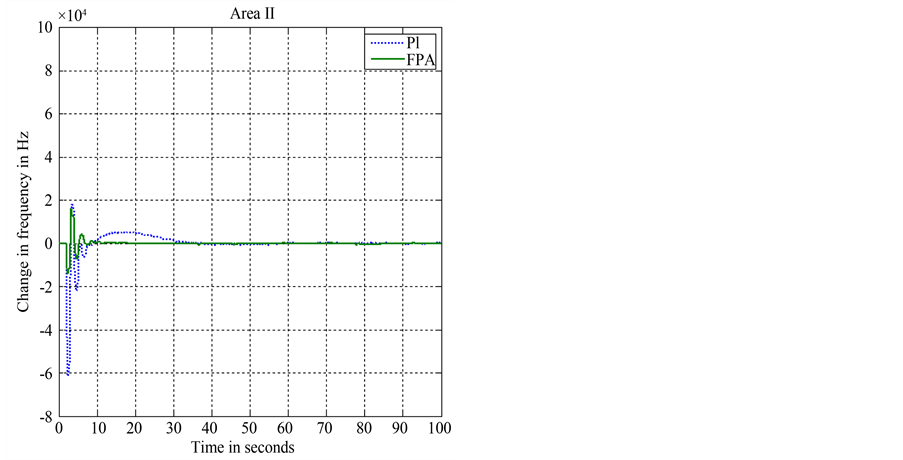
 (b) (c)
Figure 5. (a) Change in Frequency area 1 in (Hz). (b) Change in Frequency area 2 in (Hz). (c) Change in tie line in (pu∙MW).
5.2. Case 2
Bilateral transaction, i.e. all DISCOs contracts with the GENCOs for power as per the following DPM,

GENCO participate in LFC as given by the following Apf’s i.e. ,
,  ,
,  ,
,
 and
and 
The demand of DISCOs in (pu×MW) is ΔPL1 = 0.1, ΔPL2 = 0.1, ΔPL3 = 0, and ΔPL4 = 0. As the uncontracted load is considered to be zero, ΔPUC1 = 0, ΔPUC2 = 0. Each DISCO demands 0.1 (pu∙MW) power from GENCO as shown by “cpfs” in DPM.
 (22)
(22)
Hence  (pu∙Mw). By using Equation (21)
 ,
,  ,
,  and
and 
Figures 6(a)-(c) show the dynamic response of change in frequency (Hz) for each area and the tieline power flow (pu∙Mw) between them which settles at −0.05 (pu∙Mw).
Figures 6 (a)-(c) show the comparison of PI and FPA tuned PI controller for dynamic response of change in frequency (Hz) for each area and the tie line power flow (pu∙Mw) between them which settles at −0.05 (pu∙Mw). From Figures 6(a)-(c) it reveals that FPA tuned gain values of the PI controller gives better response in terms of settling time, overshoot and undershoot.
Table 1 shows the comparison of PI and FPA tuned PI controllers for two different cases such as Pool-co
 (a)
(a)
 (b) (c)
Figure 6. (a) Change in Frequency area 1 in (Hz); (b) Change in Frequency area 2 in (Hz); (c) Change in tie line in (pu∙MW).

Table 1. Comparison of performance of the controllers: Change in frequency and tie line power flow.
and Bilateral transactions. From the table for case 1, performance of the controllers shows that, FPA_PI controller gives 84% of improvement in settling time over PI. There is lesser undershoot for FPA_PI in change in area2 whereas PI has −0.002 (Hz). Similarly FPA_PI controller gives 98% settling time of tie line when compared with PI controller.
For case2, the settling time of FPA_PI controllers is found to be 50% of improvement in settling time over PI, 20% improvement in settling time of area2 over PI and 64% improvement in settling time of tie line over PI. FPA_PI has no overshoot in the tie line power whereas PI has 0.00018 (pu∙Mw). FPA_PI settles exactly at −0.05 (pu∙Mw) and PI settles at −0.052 (pu∙Mw)
6. Conclusion
Thus, a two-area hydrothermal deregulated power system is considered, which consists of two identical reheater thermal units in one area and two identical hydro units in another area. Both the areas are connected with RFB, which acts faster than governor mechanism thereby reducing the oscillations due to load disturbances. Two different types of transactions were considered such as pool-co and bilateral transactions. Simulations were done to the system considered with a PI controller whose gain values were tuned by Ziegler- Nichols and FPA methods. Integral Square Error of the system was considered as an objective function to be minimized for tuning the gains of PI using FPA. The obtained results were compared with which FPA tuned parameters of PI which, gives better results, measured by means settling time, overshoot and undershoot when compared to PI. For the same system, the non-linearity such as Governor Dead Band, Generation Rate Constraints and Time Delay may be considered for the future work.
Cite this paper
D. Lakshmi,A. Peer Fathima,Ranganath Muthu, (2016) A Novel Flower Pollination Algorithm to Solve Load Frequency Control for a Hydro-Thermal Deregulated Power System. Circuits and Systems,07,166-178. doi: 10.4236/cs.2016.74016
References
- 1. Elgerd, O.I. (1982) Electric Energy Systems Theory: An Introduction.
- 2. Report, I.C. (1973) Dynamic Models for Steam and Hydro Turbines in Power System Studies. IEEE Transactions on Power Apparatus and Systems, PAS-92, 1904-1915.
http://dx.doi.org/10.1109/TPAS.1973.293570 - 3. Demello, F., Koessler, R.J., Agee, J., Anderson, P.M., Doudna, J.H., Fish, J.H. and Taylor, C. (1992) Hydraulic-Turbine and Turbine Control-Models for System Dynamic Studies. IEEE Transactions on Power Systems, 7, 167-179.
http://dx.doi.org/10.1109/59.141700 - 4. Christie, R.D. and Bose, A. (1996) Load Frequency Control Issues in Power System Operations after derEgulation. IEEE Transactions on Power Systems, 11, 1191-1200. http://dx.doi.org/10.1109/59.535590
- 5. Fathima, A.P. and Khan, M.A. (2008) Design of a New Market Structure and Robust Controller for the Frequency Regulation Service in the Deregulated Power System. Electric Power Components and Systems, 36, 864-883.
http://dx.doi.org/10.1080/15325000801911443 - 6. Donde, V., Pai, M.A. and Hiskens, I.A. (2001) Simulation and Optimization in an AGC System after Deregulation. IEEE Transactions on Power Systems, 16, 481-489.
http://dx.doi.org/10.1109/59.932285 - 7. Ziegler, J.G. and Nichols, N.B. (1942) Optimum Settings for Automatic Controllers. Transactions of the ASME, 64, 759-768.
- 8. Gopal, M. (2002) Control Systems: Principles and Design. Tata McGraw-Hill Education, Noida.
- 9. Aditya, S.K. and Das, D. (2001) Battery Energy Storage for Load Frequency Control of an Interconnected Power System. Electric Power Systems Research, 58, 179-185.
http://dx.doi.org/10.1016/S0378-7796(01)00129-8 - 10. Chidambaram, I.A. and Paramasivam, B. (2013) Optimized Load-Frequency Simulation in Restructured Power System with Redox Flow Batteries and Interline Power Flow Controller. International Journal of Electrical Power & Energy Systems, 50, 9-24.
http://dx.doi.org/10.1016/j.ijepes.2013.02.004 - 11. Chandrakala, V., Sukumar, B. and Sankaranarayanan, K. (2014) Load Frequency Control of Multi-Source Multi-Area Hydro Thermal System Using Flexible Alternating Current Transmission System Devices. Electric Power Components and Systems, 42, 927-934.
http://dx.doi.org/10.1080/15325008.2014.903540 - 12. Weber, A.Z., Mench, M.M., Meyers, J.P., Ross, P.N., Gostick, J.T. and Liu, Q. (2011) Redox Flow Batteries: A Review. Journal of Applied Electrochemistry, 41, 1137-1164.
http://dx.doi.org/10.1007/s10800-011-0348-2 - 13. Glover, B.J. (2007) Understanding Flowers and Flowering: An Integrated Approach (Vol. 277). Oxford University Press, Oxford, UK.
http://dx.doi.org/10.1093/acprof:oso/9780198565970.001.0001 - 14. Yang, X.S. (2012) Flower Pollination Algorithm for Global Optimization. In: Unconventional Computation and Natural Computation, Springer Berlin Heidelberg, 240-249.
http://dx.doi.org/10.1007/978-3-642-32894-7_27 - 15. Dash, P., Saikia, L.C. and Sinha, N. (2016) Flower Pollination Algorithm Optimized PI-PD Cascade Controller in Automatic Generation Control of a Multi-area Power System. International Journal of Electrical Power & Energy Systems, 82, 19-28.
http://dx.doi.org/10.1016/j.ijepes.2016.02.028 - 16. (2000) MATLAB-Simulink User Manuals. Mathworks Inc., USA.
Appendix 1
System Parameters
Rating Pri = 2000 MW, Inertia Constant Hi = 5 s, Damping Coefficient Di = 1/120 pu MW/Hz, Power System Gain Constant KPi = 120 Hz/pu MW, Power system Time constants TPi = 20s, Speed Regulation Rj = 2.4 Hz/pu MW, Governor Time Constants TGj = 0.08 s, Turbine Time Constants TTj = 0.3 s, Hydro governor KHj = 1.0, Hydro governor time constant THj = 48.7 s, Reset time of hydraulic amplifier TRj = 5s, Time constant of hydraulic amplifier T2j = 0.513 s, Time constant of hydro turbine Twj = 1 s Bias factor Bi = 0.425 pu∙MW/Hz, Tie line Power constant T12 = 0.0707, System frequency f = 60 Hz, a12 = 1, Redox Flow Battery Gain constant Krfbi = 1.8, Redox Flow Battery Time constant Trfbi = 0 s. Number of flowers = 20, Maximum iterations = 100, λ = 1.5, γ = 0.1, p = 0.8.