ABSTRACT

We study a mathematical model of biological neuronal networks composed by any finite number of non-necessarily identical cells. The model is a deterministic dynamical system governed by finite-dimensional impulsive differential equations. The statical structure of the network is described by a directed and weighted graph whose nodes are certain subsets of neurons, and whose edges are the groups of synaptical connections among those subsets. First, we prove that among all the possible networks such as their respective graphs are mutually isomorphic, there exists a dynamical optimum. This optimal network exhibits the richest dynamics: namely, it is capable to show the most diverse set of responses (i.e. orbits in the future) under external stimulus or signals. Second, we prove that all the neurons of a dynamically optimal neuronal network necessarily satisfy Dale’s Principle, i.e. each neuron must be either excitatory or inhibitory, but not mixed. So, Dale’s Principle is a mathematical necessary consequence of a theoretic optimization process of the dynamics of the network. Finally, we prove that Dale’s Principle is not sufficient for the dynamical optimization of the network.

1. Introduction

Based on experimental evidence, Dale’s Principle in Neuroscience (see for instance [1,2]) postulates that most neurons of a biological neuronal network send the same set of biochemical substances (called neurotransmitters) to the other neurons that are connected with them. Most neurons release more than one neurotransmitter, which is called the co-transmission” phenomenon [3,4], but the set of neurotransmitters is constant for each cell. Nevertheless, during plastic phases of the nervous systems, the neurotransmitters are released by certain groups of neurons change according to the development of the neuronal network. This plasticity allows the network perform diverse and adequate dynamical responses to external stimulus: Evidence suggests that during both development (in utero) and the postnatal period, the neurotransmitter phenotype of neurons is plastic and can be adapted as a function of activity or various environmental signals [4]. Also a certain phenotypic plasticity occurs in some cells of the nervous system of mature animals, suggesting that a dormant phenotype can be put in play by external inputs [4].

Some mathematical models of the neuronal networks represent them as deterministic dynamical systems (see for instance [5-8]). In particular, the dynamical evolution of the state of each neuron during the interspike intervals, and the dynamics of the bursting phenomenon, can be modelled by a finite-dimensional ordinary differential equation (see for instance [8,9] and in particular [10] for a mathematical model of a neuron as a dynamical system evolving on a multi-dimensional space). When considering a network of many neurons, the synaptical connections are frequently modelled by impulsive coupling terms between the equations of the many cells (see for instance [7,11-13]). In such a mathematical model, Dale’s Principle is translated into the following statement:

Dale’s Principle: Each neuron is either inhibitory or excitatory. We recall that a neuron is called inhibitory (resp. excitatory) if its spikes produce, through the electro-biochemical actions that are transmitted along the axons of, only null or negative (resp. positive) changes in the membrane potentials of all the other neurons of the network. The amplitudes of those changes may depend on many variables. For instance, they may depend on the membrane instantaneous permeability of the receiving cell. But the sign of the postsynaptical actions is usually only attributed to the electro-chemical properties of the substances that are released by the sending cell. In other words, the sign depends only on the set of neurotransmitters that are released by. Since this set of substances is fixed for each neuron (if satisfies Dale’s Principle), the sign of its synaptical actions on the other neurons is fixed for each cell, and thus, independent of the receiving neuron.

In this paper we adopt a simplified mathematical model of the neuronal network with a finite number of neurons, by means of a system of deterministic impulsive differential equations. This model is taken from [11,13], with an adaptation that allows the state variable of each cell be multidimensional. Precisely is a vector of finite dimension, or equivalently, a point in a finite-dimensional manifold of an Euclidean space. The finite dimension of the state variable is larger or equal than 1, and besides, may depend on the neuron. 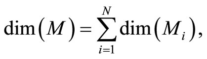The dynamical model of the network is the solution of a system of impulsive differential equations. This dynamics evolves on a product manifold whose dimension is the sum of the dimensions of the state variables of its neurons.

We do not assume a priori that the neurons of the network satisfy Dale’s Principle. In Theorem 16 we prove this principle a posteriori, as a necessary final consequence of a dynamical optimization process. We assume that during this process, a plastic phase of the neuronal network occurs, eventually changing the total numbers of neurons and synaptical connections, but such that the graph-scheme of the synaptic connections among groups of mutually identical cells remains unchanged. We assume that a maximal amount of dynamical richness is pursued during such a plastic development of the network. Then, by means of a rigourous deduction from the abstract mathematical model, we prove that, among all the mathematically theoretic networks of such a model, those exhibiting an optimal dynamics (i.e. the richest or the most versatile dynamics) necessarily satisfy Dale’s Principle (Theorem 16).

The mathematical criteria to decide the dynamical optimization is the following: First, in Definition 9, we classify all the theoretic neuronal networks (also those that hypothetically do not satisfy Dale’s Principle) into non countably many equivalence classes. Each class is a family of mutually equivalent networks, with respect to their internal synaptical connections among groups of cells (we call those groups of cells synaptical units in Definition 6). Second, in Definitions 11 and 14, we agree to say that a network has an  optimal dynamics conditioned to its class, if the dynamical system modelling any other network in the same class as, has a space of orbits in the future that is a subset of the space of orbits of. In other words, is the network capable to perform the richest dynamics, namely, the most diverse set of possible evolutions in the future among all the networks that are in the same class.

RESULTS TO BE PROVED

In Theorem 15 we prove that the theoretic dynamical optimum exists in any equivalence class of networks that have isomorphic synaptical graphs.

In Main Theorem 16 we prove that such an optimum is achieved only if the network satisfies Dale’s Principle.

In Main Theorem 17 we prove that the converse of Theorem 16 is false: Dale’s Principle is not sufficient for a network exhibit the optimal dynamics within its synaptical equivalence class.

The results are abstract and theoretically deduced from the mathematical model. They are epistemologically suggestive since they give a possible answer to the following question:

Epistemological question: Why does Dale’s Principle hold for most cells in the nervous systems of animals?

Mathematically, the hypothesis of searching for an optimal dynamics implies (through Theorem 16) that at some step of the optimization process all the cells must satisfy Dale’s Principle. In other words, this principle would be a consequence, instead of a cause, of an optimization process during the plastic phase of the network. This conclusion holds under the hypothesis that the dynamical optimization (i.e. the maximum dynamical richness) is one of the natural pursued aims during a certain changeable development of the network.

Finally, we notice that the converse of Theorem 16 is false: there exist mathematical examples of simple abstract networks whose cells satisfy Dale’s Principle but are not dynamically optimal (Theorem 17). Thus, Dale’s Principle is necessary but not sufficient for the dynamical optimization of the network.

Structure of the paper and purpose of each section: In Section 2, we write the hypothesis of Main Theorems 16 and 17. This Section is necessary because the proofs of the theorems are deduced from the hypothesis. In other words, their statements could be false if not all the hypothesis holded.

From Section 3 to 6 we prove Main Theorem 16. The proof is developed in four steps, one in each separate section. The first step (Section 3) is devoted to prove the intermediate result of Proposition 7. The second step (Section 4) is deduced from Proposition 7. The third step (Section 5) is logically independent from the first and second steps, and is devoted to obtain the two intermediate results of Proposition 13 and Theorem 15. Section 6 exposes the fourth step (the end) of the proof of Main Theorem 16, from the logic junction of the previous three steps, using the intermediate results (Propositions 7 and 13, and Theorem 15).

On the one hand, the intermediate results (Propositions 7 and 13, and Theorem 15) are necessary stages in the logical process of our proof of Main Theorem 16 which ends in Section 6. In fact, Theorem 16 establishes that, if there exists a dynamical optimum within each synaptical equivalence class of networks, this optimal network necessarily satisfy Dale’s Principle. But this result would be void if we did not prove (as an intermediate step), that a dynamically optimal network exists (Theorem 15). It would be also void if we did not prove that the synaptical equivalence classes of networks exist (Definition 9). The synaptical equivalence classes of networks could not been defined if the inter-units graph of the network did not existed (Definition 8). And these graphs exist as an immediate corollary of Proposition 7. So, Proposition 7 must be proved as an intermediate step for our final purpose. Finally, the end of the proof of Main Theorem 16 argues by contradiction: if the dynamically optimal network did not satisfy Dale’s Principle, then Proposition 13 would be false. So, we need first, also as an intermediate step, to prove Proposition 13.

On the other hand, to prove all the required intermediate results, we need some other (previous) mathematical statements from which we deduce the intermediate results. So, we start posing all the previous mathematical statements (obtaining them from the general hypothesis of Section 2), in a series of mathematical definitions, comments and remarks that are at the beginning of Sections 3, 4 and 5.

In Section 7, we end the proof of Main Theorem 17 stating that Dale’s Principle is not sufficient for the dynamical optimization. Its final statement is proved by applying directly some of the definitions, intermediate results and examples of Sections 3, 4 and 5 (in particular, those of Figures 1-3).

Finally, in Section 8 we write the conclusions obtained from all the mathematical results that are proved along the paper.

2. The Hypothesis (The Model by a System of Impulsive Differential Equations)

We assume a simplified (but very general) mathematical model of the neuronal network which is defined along this section. The model, up to an abstract reformulation, and a generalization that allows any finite dimension for the impulsive differential equation governing each neuron, is taken from [11] and [13]. In the following subsections we describe the mathematical assumptions of this model:

2.1. Model of an Isolated Neuron

Each neuron, while it does not receive synaptical actions from the other cells of the network, and while its membrane potential is lower than a (maximum) threshold level, and larger than a lower bound, is assumed to be governed by a finite-dimensional differential equation of the form

(1)

where is time, is a finite-dimensional vector whose components are real variables that describe the instantaneous state of the cell, and is a Lipschitz continuous function giving the velocity vector of the changes in the state of the cell, as a function of its instantaneous vectorial value. The function is the so called vector field in the phase space of the cell. This space is assumed to be a finite dimensional compact manifold. The advantages of considering that (not necessarily 1) are, among others, the possibility of showing dynamical bifurcations between different rythms and oscillations that appear in some biological neurons [10], that would not appear if the mathematical model of all the neurons were necessarily onedimensional.

One of the components of the vectorial state variable (which with no loss of generality we take as the first component) is the instantaneous membrane potential of the cell.

In the sequel, we denote and

In addition to the differential equation (1), it is assumed the following spiking condition [9]: If there exists an instant such that the potential equals the  threshold level, then. In brief, the following logic assertion holds, by hypothesis:

(2)

Here, is the reset value. It is normalized to be zero after a change of variables, if necessary, that refers the difference of membrane potential of the cell to the reset value. A more realistic model would consider a positive relatively short time-delay between the instant when the membrane potential arrives to the threshold level, and the instant for which the potential takes its reset value. During this short time-delay, the membrane potential shows an abrupt pulse of large amplitude, which is called spike of the neuron. The impulsive simplified model approximates the spike to an abrupt discontinuity jump, by taking the time-delay equal to zero. Then, the spike becomes an instantaneous jump of the membrane potential from the level to the reset value which occurs at according to condition (2).

We denote by the Dirac delta supported on. Namely (via the abstract integration theory with respect to the Dirac delta probability measure) denotes a discontinuity step that occurs on the potential at each instant such that. In other words:

and so

After the above notation is adopted, the dynamics of each cell (while isolated from the other cells of the network) is modelled by the following impulsive differential equation:

(3)

In the above equality is the jump vector with dimension equal to the dimension of the state variable. Namely, at each spiking instant, only the first component (the membrane potential) is abruptly reset, since the jump vector has all the other components equal to zero.

Strictly talking, the Equation (3) is not a differential equation, but the hybrid between the differential equation plus a rule, denoted by. This impulsive rule imposes a discontinuity jump of amplitude vector in the dependence of the state variable on. Therefore, is not continuous, and thus it is not indeed differentiable. It is in fact discontinuous at each instant such that, i.e. when the Dirac delta is not null.

Nevertheless, the theory of impulsive differential equations follows similar rules than the theory of ordinary differential equations. It was early initiated by Milman and Myshkis [14], cited in [15]. In particular, the existence and uniqueness of solution for each initial condition, and theorems of stability, still hold for the impulsive differential Equation (3), as if it were an ordinary differential equation [14,15].

2.2. Model of the Synaptical Interactions among the Neurons

The synaptical interactions are modelled by the following rule: If the membrane potential of some neuron arrives to (or exceeds) its threshold level at instant, then the cell sends an action to the other neurons. In particular may be zero if no synaptical connection exists from the cell to the cell. This action produces a discontinuity jump in the membrane potential. We denote by the signed amplitude of the discontinuity jump on the membrane potential of the neuron, which is produced by the synaptical action from the neuron, when spikes. The real value may depend on the instantaneous state of the receiving neuron just before the synaptic action from neuron arrives. For simplicity we do not explicitly write this dependence. Thus, the symbol denotes a real function of, which we assume to be either identically null or with constant sign.

We denote by the discontinuity jump vector, with dimension equal to the dimension of the variable state of the cell. In other words, the discontinuity jump in the instantaneous vector state of the cell, that is produced when the cell spikes, is null on all the components of except the first one, i.e. except on the membrane potential of the neuron. In formulae:

(4)

Thus, the dynamics of the whole neuronal network is modelled by the following system of impulsive differential equations:

(5)

where is the number of cells in the network.

Definition 1 (Excitatory, inhibitory and mixed neurons) The synapses from cell to is called excitatory if and it is called inhibitory if. If then there does not exist synaptical action from the cell to the cell. A neuron is called excitatory (resp. inhibitory) if (resp.) for all such that. The cell is called mixed if it is neither excitatory nor inhibitory. Dale’s Principle (which we do not assume a priori to hold) states that no neuron is mixed.

Remark 2 It is not restrictive to assume that no cell is indifferent, namely no cell sends null synaptical actions to all the other cells, i.e.

In fact, if there existed such a cell, it would not send any action to the other cells of the network. So, the global dynamics of the network is not modified (except for having one less variable) if we take out the cell from.

All along the paper we assume that the network has at least 2 neurons and no neuron is indifferent.

2.3. The Refractory Rule

To obtain a well defined deterministic dynamics from the system (5), other complementary assumptions are adopted by the model. First, a refractory phenomenon (see for instance [16, page 725]) is considered as follows: If some fixed neuron spikes at instant, then its potential is reset to zero becoming indifferent to the synaptical actions that it may receive (at the same instant) from the other neurons. Second, if for some fixed neuron at some instant, the sum of the excitatory actions that simultaneously receives from the other neurons of the network, is larger or equal than, then itself spikes at instant, regardless whether or not. In this case, at instant the cell sends synaptical actions to the other neurons of the network, and then, the respective potentials will suffer a jump at instant. This process may make new neurons to spike in an avalanche process (see [13]). This avalanche is produced instantaneously, when some excitatory neuron spontaneously arrived to its threshold level. But due to the refractory rule, once each neuron spikes, its membrane potential refracts all the excitations or inhibitions that come at the same instant. So, the avalanche phenomenon is produced instantaneously, but includes each neuron at most once. Then, each interaction term in the sum at right of Equation (5) is added only once at each spiking instant.

3. First Step of the Proof (Graphs, Parts and Units)

The purpose of this section is to prove Proposition 7 and to state the existence of an Inter-units Graph (Definition 8). These are intermediate results (the first step) of the proof of Main Theorems 16 and 17. We will prove these intermediate results by logical deduction from several previous statements and hypothesis. So, we start by including the needed previous statements in the following series of mathematical definitions:

Let be a network of neurons, according to the model defined in Section 2.

Definition 3 (The Network’s Graph) We call a directed and weighted graph the graph of the network if the vertices of are the cells of, each edge of, corresponds to each nonzero synaptical action from the cell to the cell and conversely, and has weight. (See the example of Figure 1.)

To unify the notation, we agree:

• denotes either the network or its graph;

• is either a cell of or a node of the graph;

• denotes either the synaptical action from to, or the weight of the edge in the graph, or this edge itself.

Definition 4 (Structurally identical cells) Two different cells are structurally identical if in the respective differential Equations (3), , and for all. These conditions imply that the dynamical systems that governs neurons and are the same. So, their future dynamics may differ only because their initial states and may be different. Note that, if and are structurally identical, then by definition, the edges of the graph at the receiving nodes and (from any other fixed sending node) are respectively equally weighted by. Nevertheless, the edges from and, as sending nodes of the network, are not necessarily identically weighted, i.e. may be different from.

In Figure 1 we represent a graph with three mutually identical cells 1, 2 and, provided that in the Equation (3) and for. Besides, the graph has two other nodes, which corresponds to the neurons and. The cells and are not mutually identical because the synaptical actions that they receive from the other cells are not equal.

The above definitions and the following ones are just mathematical tools, with no other purpose than enabling us to prove Theorems 16 and 17. They are not aimed to explain physiological or functional roles of subsets of real biological neurons in the brain or in the nervous system. Nevertheless, it is rather surprising that the following abstract mathematical tools, which we include here just to prove Theorems 16 and 17, have indeed a resemblance with concepts or phenomena that are studied by Neuroscience. In particular, the following Definitions 5 and 6 of homogeneous part and synaptical unit of a neuronal network, are roughly analogous to the concepts of regions, subnetworks or groups of many similar neurons, characterized by a certain structure and a collective physiological role. For instance some subnetworks or layers of biological or artificial neurons are defined according to the role of their synaptical interactions with other subnetworks or layers [17].

Definition 5 (Homogeneous Part) An homogeneous part of the neuronal network is a maximal subset of cells of the network that are mutually pairwise identical (cf. Definition 4). As a particular case, we agree to say that an homogeneous part is composed by a single neuron when no other neuron is structurally identical to. In Figure 1 we draw the graph of a network composed by three homogeneous parts and. The homogeneous part is composed by the three identical neurons 1, 2 and 3, provided that and for. The homogeneous parts and have a single neuron each because for some (for instance for).

Definition 6 Synaptical Unit A synaptical unit is a subset of an homogeneous part of a neuronal network such that:

• For any neuron there exists at most one neuron such that.

• is partitioned in a minimal number of sets possessing the above property.

In particular, a synaptical unit may be composed by a single neuron. This occurs, for instance, when for some neuron and for any neuron the synaptical interaction from to is nonzero. In Figure 1 we draw the graph of a network composed by three homogeneous parts, and such that: is composed by three identical neurons 1, 2 and 3, that form two synaptical units and. In fact, the cells and can not belong to the same unit because there exist nonzero actions departing from both of them to neuron. One can also form the two synaptical units of by defining and. The homogeneous part is composed by a single neuron, and thus, it is a singe synaptical unit. Analogously is composed by a single neuron, and thus it is a single synaptical unit. The total number of neurons of the network in Figure 1 is 5, the total number of synaptical units is 4, the total number of homogeneous parts is 3, the total number of nonzero synaptical interactions among the neurons is 9, but the total number of synaptical interactions among different homogeneous parts is only 5 (see Figure 2).

When a synaptical unit has more neurons, the following quotient diminishes: is the number of synaptical connections departing from the cells of divided by the total number of neurons of. In fact, by Definition 6, for each synaptical unit there exists at most one nonzero synaptical action to any other fixed neuron of the network, regardless how many cells compose. So, if we enlarge the number of cells in, the number of nonzero synaptical actions departing from the cells of remains constant. Thus, the quotient diminishes. Although this quotient becomes smaller when the number of neurons of the synaptical unit enlarges, in Theorem 15 we will rigourously prove the following result:

The dynamical system governing a neuronal network with the maximum number of neurons in each of its synaptical units, is the richest one, i.e. will exhibit the largest set of different orbits in the future, and so it will be theoretically capable to perform the most diverse set of processes.

The following result proves that any neuronal network, according to the mathematical model of Section 2, is decomposed as the union of at least two homogeneous parts, and each of these parts is decomposed into pairwise disjoint synaptical units. It also states the existence of an upper bound for the number of neurons that any synaptical unit can have.

Proposition 7 (Intermediate result in the proof of Main Theorems 16 and 17)

Let be any network according to the mathematical model defined in Section 2. Then:

1) The set of neurons of is the union of exactly pairwise disjoint homogeneous parts.

2) Each homogeneous part is the union of a positive finite number of pairwise disjoint synaptical units.

3) The total number of neurons of each synaptical unit is at least one and at most.

4) For each synaptical unit and for each homogeneous part there exists a unique real number that satisfies the following properties:

if and only if for all and for all. In particular if.

if and only if for one and only one neuron and for all, and for all and all such that.

Proof: 1) We denote if the cells and are structurally identical according to Definition 4. We add the rule for any cell. Thus, is an equivalence relation. From Definition 5 the classes of neurons are the homogeneous parts of the network.

Since the equivalence classes of any equivalence relation in any set determine a partition of this set, then the network, as a set of neurons, is the union of its pairwise disjoint homogeneous parts. Denote by the total number of different homogeneous parts that compose the network. Let us prove that. In fact, if were equal to 1, then, by Definition 4, for any pair of cells, contradicting the assumption that no cell is indifferent (see the end of Remark 2). We have proved Assertion 1).

2) Fix an homogeneous part, and fix some neuron. Consider the set of neurons. The set is nonempty because the cell is not indifferent (see Remark 2). Choose and fix a neuron. We discuss two cases: either for all, or the set is nonempty.

In the first case, for each neuron the singleton (formed by the single element), satisfies Definition 6. Thus, is a synaptical unit for all and assertion 2) is proved.

In the second case, consider the set . Consider also (if they exist) all the singletons where is such that. These latter sets satisfy Definition 6 and, thus, they are pairwise disjoint synaptical units, which are also disjoint with. Besides, their union with compose. So, it is now enough to prove that is also the union of pairwise disjoint synaptical units.

Now, we choose and fix a neuron such that. (Such a neuron exists because). By construction of the set, we have. But, since the neuron is not indifferent, there exists. So, we can repeat the above argument putting in the role of, in the role of, and in the role of.

Since the number of neurons is finite, after a finite number of steps (repeating the above argument at each step), we obtain a decomposition of into a finite number of pairwise disjoint sets that are synaptical units, ending the proof of Assertion 2).

3) Let be a synaptical unit. By Definition 6, where is an homogeneous part of the set of neurons. By Assertion 1) there are exactly other homogeneous parts. From Definitions 4 and 5, for any fixed for all. So, for each we denote

Since any neuron is not indifferent, there exists at least one homogeneous part such that. Besides, applying Definition 6, for each homogeneous part, there exists at most one neuron such that. The last two assertions imply that there is a one-to-one correspondence (which is not necessarily surjective) from the set of neurons in to the set of homogeneous parts that are different from. Then, the number of neurons in is not larger than the number of existing homogeneous parts, i.e. it is not larger than. We have proved Assertion 3).

4) Fix an arbitrary synaptical unit (where is the homogeneous part that contains) and an arbitrary homogeneous part (in particular, may be). As in the above proof of Assertion 3), for each neuron it is defined such that for all. By Definition 6, either for all, or for one and only one cell. In the first case we define and in the second case we define. By construction, Assertion (iv) holds: in particular, from Definitions 4 and 5, we have for all and for all. So, if.□

Definition 8 (Inter-units graph—Intermediate result in the proof of Theorems 16 and 17) As a consequence of Proposition 7 the graph of a neuronal network can be represented by a simpler one, which we call the inter-units graph. This is, by definition, the graph whose nodes are not the cells but the synaptical units. Each directed and weighted edge in the inter-units graph, links a synaptical unit with the synaptical unit . It is weighted by the synaptical action. For instance, the network of Figure 1 is represented by the inter-units graph of Figure 2.

Interpretation: The inter-units graph of a neuronal network, according to Definition 8, recovers the essential anatomy of the spatial distribution of the synaptical connections of the network, among groups of mutually identical cells (the so called synaptical units). This description, by means of the inter-units graph, recalls experimental studies on the synaptical activity of some neuronal subnetworks of the brain. For instance, in [17], Megas et al. study the spatial distribution of inhibitory and excitatory synapses inside the hippocampus.

Each synaptical unit acts, in the inter-units graph, as if it were a single neuron. The spatial statical structure of groups of synaptical connections is the only observed object by this graph. Besides, the inter-units graph does not change if the number of neurons composing each of the many synaptical units, change. In the following section, we will condition the study of the networks to those that have mutually isomorphic inter-units graphs, i.e. they have the same statical structure of synaptical connections among groups of identical cells.

In Section 5, we will look on the dynamical responses of the network that have the same (statical) inter-units graph of synaptical connections. Any change in the number of neurons will change the space of possible initial states, and so the space of possible orbits and the global dynamics. So, among all the networks that have isomorphic inter-units graphs, the network with more neurons should, a priori, exhibit a larger diversity of theoretic possible dynamical responses to external stimulus.

For instance, two identical neurons and in a synaptical unit define a space of initial states (and so of orbits) that is composed by all the pairs of vectors in the phase space of each neuron. But three identical neurons, and in, define a space of initial states composed by all the triples of vectors. So, the diversity of orbits that a neuronal network can exhibit, enlarges if the number of neurons of each synaptical unit enlarges. In Section 5, we will study the theoretical optimum in the dynamical response of a family of networks that are synaptical equivalent. We will prove that this optimum exists and that it is achieved when the network has the maximum number of cells (Theorem 15).

4. Second Step of the Proof (Synaptical Equivalence between Networks)

The purpose of this section is to prove the existence of an equivalence relation (Definition 9) in the space of all the neuronal networks modelled by the mathematical hypothesis of Section 2. This is the intermediate result in the second step of the proof of Main Theorems 16 and 17. We will deduce this intermediate result from the previous ones obtained in Section 3.

Let and be two neuronal networks according to the model defined in Section 2. Denote:

and the numbers of neurons of and respectively,

and a (general) neuron of and respectively,

and the respective numbers of homogeneous parts of and, according to Definition 5.

and the respective numbers of synaptical units according to Definition 6.

and a (general) homogeneous part of and respectively.

and a (general) synaptical unit of and respectively.

the synaptical weights, according to part (iv) of Proposition 7, of and respectively.

Definition 9 (Synaptically equivalent networks— Intermediate result in the proof of Main Theorems 16 and 17)

We say that and are synaptically equivalent if:

• , according to the above notation.

• There exists a one-to-one and surjective correspondence from the set of synaptical units of and the set of synaptical units of such that

where is the homogeneous part of the network whose synaptical units are the images by of the synaptical units that compose.

• For any synaptical unit of

where and are the second terms of the impulsive differential Equations (3) that govern the dynamics of the neurons and, respectively.

In other words, the networks and are synaptically equivalent, if there exists an isomorphism between their respective inter-units graphs such that all the neurons in the unit of the network are structurally identical to all the neurons in the unit of the network.

For example, let us consider the network of Figure 3. Assume that, in the respective impulsive differential equations (3). Also assume that for and. Then, the network has homogeneous parts Analogously to the example of Figure 1, the part of the network is composed by two synaptical units and, and the part is composed by a single synaptical unit. Finally, the part of the network of Figure 3 is composed by a single synaptical unit.

Assume that the interactions and of the networks and of Figures 1 and 3 respectively, satisfy the following properties:

for all such that,

for all

,

.

Then, the inter-units graph of Figure 2 also corresponds to the network. So, the networks and of Figures 1 and 3 are synaptically equivalent.

We note that, for synaptically equivalent networks, the number of neurons, and also the number of nonzero synaptical interactions, may vary. For instance, the networks of Figures 1 and 3 are synaptically equivalent, but their respective total numbers of of neurons and of synaptical interactions are mutually different.

Comments: The equivalence relation between networks and, according to Definition 9, implies that both and will have exactly the same dynamical response (i.e. they will follow the same orbit), provided that, for any dynamical unit of, the initial states of all the neurons in are mutually equal and also equal to the initial states of all the neurons in the dynamical unit of the other network. In fact, since the impulsive differential Equations (3) that govern the dynamics of all those neurons coincide, and since the synaptical jumps that each of those neurons receive from the other neurons of its respective network also coincide, their respective deterministic orbits in the future must coincide if the initial states are all the same.

Nevertheless, if not all those initial states are mutually equal, for instance if some external signal changes the instantaneous states of some but not all the neurons in a synaptical unit, then their respective orbits will differ, during at least some finite interval of time. In this sense, each synaptical unit with more than one neuron, is a group of identical cells that distributes the dynamical process among its cells, i.e. it has the capability of dynamically distributing the information.

In brief, two synaptically equivalent networks have, as a common feature, the same statical configuration or anatomy of the synaptical interactions between their units (i.e. between groups of identical cells, equally synaptically connected). Then, both networks would evolve equally, under the hypothetical assumption that all the initial states of the neurons of their respective synaptical units coincided. But the two networks may exhibit qualitatively different dynamical responses to external perturbations or signals, if these signals make different the instantaneous states of different neurons in some synaptical unit. Such a difference produces a diverse distribution of the dynamical response among the cells.

5. Third Step of the Proof (Dynamically Optimal Networks)

The purpose of this section is to prove Proposition 13 and Theorem 15. These are intermediate results (the third step) of the proof of Main Theorems 16 and 17. We will prove these intermediate results by logical deduction from several previous statements and hypothesis. So, we start by including the needed previous statements in the following series of mathematical definitions, remarks and notation agreements:

We condition the study to the networks of any fixed single class, which we denote by, of synaptically equivalent networks according to Definition 9. In this section we search for networks exhibiting an optimum dynamics conditioned to.

Notation:

We consider the mathematical model of a general neuronal network, given by the system (5) of impulsive differential equations. We denote by

the instantaneous state of the network at instant, where is the number of neurons of the network, and is the instantaneous state of the neuron. Since by hypothesis evolves on a finite-dimensional compact manifold, the state of the network evolves on the finite-dimensional compact product manifold, defined by the following equality:

In other words, is the cartessian product of the manifolds. Then

(6)

Definition 10 (Dynamics of the network) Consider any initial state

of the network, i.e. is the state of the neuron at the instant.

The solution of the system (5) of impulsive differential equations that govern the dynamics of, exists and is unique, provided that the initial condition is given (see for instance [14], cited in [15]). We denote:

and call the (deterministic) dynamical system (or, in brief, the dynamics) associated to the network. It is an autonomous deterministic dynamical system.

For any autonomous deterministic dynamical system (also if it were not modelled by differential equations), we have the following properties:

So, for any fixed instant the state plays the role of a new initial state, from which the orbit

evolves for time. This orbit coincides with the piece of orbit (for time) that had the initial state.

Definition 11 (Partial Order in)

Let and be two networks in and denote by and the dynamics of and respectively. Denote by and the compact manifolds where and respectively evolve.

We say that is dynamically richer than, and write

if there exists a continuous and one-to-one (non necessarily surjective) mapping

such that

(7)

for any initial state.

In other words, if and only if the dynamical system of is a subsystem of the dynamical system of, up to the continuous change of the state variables.

From Definition 11 it is immediately deduced the following assertion:

and if and only if their respective dynamical systems and are topologically conjugated.

This means that the dynamics of and are the same topological dynamical system, up to an homeomorphic change in their variables which is called a conjugacy. So, we deduce:

is a partial order in the class of synaptically equivalent networks up to conjugacies.

As an example, assume that the numbers and of neurons of and satisfy. Then, . Define the function by:

If this function satisfies Equality (7), then each orbit of the dynamical system of, is identified with one orbit of the dynamics of. Along this orbit, each two consecutive identical neurons have the same initial states, and thus also have coincident instantaneous states for all. Nevertheless, the whole dynamics of the network also includes many other different orbits, which are obtained if the initial states of some pair of consecutive identical neurons of are mutually different.

Remark 12 From Definition 11, since is continuous and one-to-one, we deduce that the image is a submanifold of which is homeomorphic to. This is a direct application of the Domain Invariance Theorem (see for instance [18]). Therefore:

Besides,. So, contains the submanifold that has the same dimension than. We deduce the following statement:

(8)

In extensum:

If the dynamics of is richer than the dynamics of, then the dimension of the manifold where the dynamics of evolves, is larger or equal than the dimension of the manifold where the dynamics of evolves.

From the above remark we deduce the following result:

Proposition 13 (Intermediate result in the proof of Main Theorems 16 and 17)

If and are synaptically equivalent and if, then the number of neurons of is larger or equal than the number of neurons of.

Proof: Both networks are synaptically equivalent; so, each neuron of is structurally identical to some neuron (which we still call) of. This implies that the finite dimension of the variable in the network is equal to the finite dimension of the corresponding variable in the network. Thus,

(9)

After Equality (6) applied to the networks and respectively, we obtain:

(10)

(11)

where and are the number of neurons of and respectively. From Inequality (8) we have:

Finally, substituting (10) and (11), we obtain:

and joining with (9) we conclude, as wanted.

Definition 14 (Dynamically optimal networks) We say that a network is a dynamical optimum conditioned to the synaptical equivalence class (i.e. within the class) if for all.

Theorem 15 (Existence of the dynamical optimum

Intermediate result in the proof of Main Theorems 16 and 17)

For any class of synaptically equivalent neuronal networks there exists a dynamical optimum network conditioned to. This optimal network has the maximum number of cells among all the networks of the class.

Proof: The class of synaptically equivalent networks is characterized by the numbers and of homogeneous parts and synaptical units respectively, and by the real values of the synaptical connections between the dynamical units and the homogeneous classes.

For each dynamical unit, we denote by the number of homogeneous classes such that. Thus, because each cell is not indifferent, and so, there exists at least one nonzero synaptical action departing from. (Recall that by Definitions 4 and 5, the nonzero synaptical actions only exist between cells belonging to different homogeneous parts.)

Construct a network as follows:

First, compose each dynamical unit with exactly cells. Then, there exists a surjective one-to-one correspondence between the set of cells and the set of homogeneous parts satisfying .

Second, define the synaptical connections departing from each cell of each dynamical unit, by the following equalities:

(12)

(13)

We will prove that the network such constructed is dynamically optimal within the class:

Fix any network. Consider the dynamical systems and corresponding to the networks and respectively. Denote by and the compact manifolds where and respectively evolve. According to Definition 11, to prove that it is enough to construct a continuous oneto-one mapping satisfying Equality (7).

Let. For any cell, the initial state is a component of. Let us define satisfying Equality (7). To do so, we must define the initial state of any cell of the network.

So, fix. Denote by the synaptical unit to which belongs, and denote by the unique homogeneous class of the network satisfying (12). We denote

(14)

where and

Since is synaptical equivalent to (because both networks and belong to the same class), we apply Definition 9 to deduce the following equalities:

(15)

From Definition 6, there exists a unique cell such that

(16)

Summarizing, for any fixed neuron we have constructed a unique cell such that Equalities (14), (15) and (16) hold. In other words, we have constructed a mapping, defined from the synaptical equivalence between the networks and, such that:

(17)

where is the unique homogeneous class in satisfying (12).

Assertion A: The mapping transforms each cell of the network into the cell in the network, which is structurally identical to.

In fact, assertion A follows from the fact that and are synaptically equivalent (cf. Definition 9) and from Equality (17).

Let us prove that is surjective. In fact, for each, there exists at least one homogeneous part such that, because is not indifferent. By Definition 9, where is a one-to-one and surjective transformation between the homogeneous parts of and. Therefore, there exists a unique homogeneous part of such that, where, and. By construction of the network, if, then there exists a unique such that. Then, we deduce that. Joining with (17), and recalling that for each synaptical unit there exists at most one cell such that, we deduce. This proves that is surjective.

We define the initial state of the cell by

and the mapping by

(18)

The mapping is continuous because the components of are components of. Thus, small increments in the components of imply small increments in the components of. Besides, the mapping is one-to-one (but non necessarily surjective). In fact, if then, at least one component of differs from the respective component of. Since is surjective, there exists such that. So, applying Equality (18) we obtain, where. Thus proving that is one-to-one.

To end the proof of the first part of Theorem 15, it is now enough to check that the mapping satisfies Equality (7):

From Equality (18) and from the surjectiveness of, for each initial state of the network, and for each neuron, the corresponding set of neurons have initial states which equal. Besides, from Assertion A, and are structurally identical. Now, we consider Equalities (14), (15) and (17), applied to any neuron and, in the respective roles of and. We deduce that the synaptical interaction jumps that receives from any other neuron coincides with the synaptical interaction jumps that receives from in the network. Therefore, both and satisfy the same impulsive differential equation (5). Besides, their respective initial conditions and coincide, due to Equality (18). Since the solution of the impulsive differential Equation (5) that satisfies a specified initial condition is unique, we deduce the following statement:

For any instant the state coincides with the instantaneous state, where.

Recalling Definition 10 of the dynamics and of the networks and respectively, we deduce:

Applying again Equality (18), which defines the mapping for each fixed instant as the new initial state, we conclude

proving Equality (7), as wanted.

We have proved that for all. Thus, in each synaptical equivalence class there exists a network that is the dynamical optimum conditioned to.

Now, let us prove the second part of Theorem 15. We have to show that the number of neurons in is the maximum number of neurons of all the networks in the class. In fact, since, after Proposition 13 we get, where is the number of neurons of, for all.

6. End of the Proof of Dale’s Principle

Let be the set of all the neuronal networks according to the mathematical model defined in Section 2. Let be a fixed class of synaptically equivalent networks. The purpose of this section is to end the proof of the following Main Theorem of the paper:

Theorem 16 (Dale’s Principle is necessary for the dynamical optimization)

If is the dynamical optimum network conditioned to, then all the neurons of satisfy Dale’s Principle.

Namely, any neuron of is either inhibitory or excitatory.

End of the proof of Theorem 16: Let be the dynamical optimum among the networks in. Therefore,

Thus, applying Proposition 13, the numbers and of neurons in and respectively, satisfy

(19)

Denote by the synaptical action from the neuron to the neuron in, for any Assume by contradiction that there exists a neuron which is mixed, according to Definition 1. Let us fix such a value of. Now, we construct a new network as follows:

First, include in all the neurons, in particular. Define in the synaptical interactions as follows:

Second, add one more neuron in, say the - th. neuron, which we make, by construction, structurally identical to the -th. neuron. Define

The new neuron is not indifferent in the network because is mixed in. (So, there exists such that.)

It is immediate to check that is synaptically equivalent to. In fact, all the neurons, except the added one -th. cell in, are respectively structurally identical in the networks and. Besides, all the synaptical interactions, except those that depart from and, are the same in both networks. Finally, also the nonzero synaptical interactions that depart from in the network, are equal, either to the synaptical interactions that depart from in (if positive), or to those that depart from the new neuron in (if negative). So, is synaptically equivalent to. In other words,. To end the proof, we note that the number of neurons of is, contradicting Inequality (19).□

7. Counter Example

The purpose of this section is to exhibit a counter-example that shows that the converse of Main Theorem 16 is false (Theorem 17).

Theorem 17 is the second Main Theorem of the paper. Its proof is deduced from the intermediate results that were previously obtained along the paper, and is ended by showing the explicit counter-example from Figures 1-3.

Theorem 17 (Dale’s Principle is not sufficient for the dynamical optimization)

There exist neuronal networks according to the mathematical model of Section 2 that satisfy Dale’s Principle and are not dynamically optimal conditioned to their respective synaptical equivalence classes.

End of the proof of Theorem 17: We will show an explicit example of a dynamical suboptimal network within a synaptical equivalence class, such that satisfies Dale’s Principle. We will exhibit such an example with neurons, but it can be repeated (after obvious adaptations) with any arbitrarily chosen number.

Consider the network of Figure 1. Assume, for instance, the following signs for the nonzero synaptical interactions:

Then, the neurons and are excitatory and the neurons 1, 3 and are inhibitory. Thus, all the neurons of the network satisfy Dale’s Principle.

As shown in Section 4, the network of Figure 3 is synaptically equivalent to the network of Figure 1. In other words, both networks and belong to the same equivalence class. Since has exactly 6 neurons and has 5 neurons, applying Proposition 13 we deduce that. Thus is not the optimal network of its class.

8. Final Comments

In Section 2 we posed the mathematical simplified (but general) model of biological neuronal networks, by a system (5) of deterministic impulsive differential equations. In its essence, this model was taken from [11] (some particular conditions of the model were also taken from [8-10,12,13] and from the bibliography therein).

On the one hand, the mathematical model is an idealized simplification of the network, because the spiking of each neuron is reduced to an instantaneous reset, without delay, of its membrane potential. Also the synaptical actions are assumed to be instantaneous and have no delay.

On the other hand, the abstract mathematical model is general, since we require neither particular formulae, nor numerical specification, nor computational algorithms for the functions, and of Equations (1), (3) and (5), nor specific values for the parameters.

In Section 3 we defined the homogeneous parts of the network, composed by mutually identical cells. The groups of neurons, which we call synaptical units, are formed by structurally identical and synaptically representative neurons. In Proposition 7 we proved that any neuronal network, according to the mathematical model described in Section 2, is decomposable in more than one homogeneous part, and that each homogeneous part is decomposable into pairwise disjoint dynamical units. Then, a simplified graph, which we called inter-units graph mathematically represents the statical structure of the synaptical connections among the groups of neurons in the network. This theoretical approach have rough similitudes with empirical research in Neuroscience [17], for which the structure of synaptical connections among groups of neurons or regions in the brain is studied, regardless how many neurons exactly compose each region.

In Section 4 we conditioned the study to a fixed family of networks that are mutually synaptically equivalent. We denote this family by, and call it a class. Even if this condition may appear as a restriction, it is not. In fact, first, any neuronal network (provided that it is mathematically modelled by the equations of Section 2), belongs to one such a class. Second, all the results that we proved along the paper stand for any arbitrarily chosen class of synpatically equivalent networks.

Each class of synaptically equivalent networks gives a particular specification for the number of synaptical units and for the inter-units graph. This specification implies a particular statical anatomy in the synaptical structure of the network, described by the different groups of mutually identical neurons (and not by the neurons themselves). Each group of neurons is a synaptical unit that has a characteristic functional role in the complex synaptical structure of the network.

Roughly speaking, a class of mutually synaptically equivalent neuronal networks works as an abstraction of the following analogous example: When a Neuroscientist studies the nervous system of certain species of animals, he is investigating a class of neuronal networks composed by a relatively large amount of particular cases that are indeed different networks (one particular case for each individual of the same species). But all the neuronal networks in that class share a certain structure, which is given, for instance, by the genetic neurological characteristics of the species. Some type of synaptical connections between particular groups of neurons with specific physiological roles, is shared by all the healthy individuals of the species. However, the exact number of neurons, and the exact number and weight of synaptical connections between particular neurons, may vary from one individual to another of the same species, or from an early age to a mature age of the same individual.

In Section 5 we studied the abstract dynamical system of any neuronal network defined by the mathematical model of Section 2, and conditioned to a certain fixed class of mutually synaptically equivalent networks. In Theorem 15 we proved that (theoretically) a dynamically optimal network exists in each class.

The proof of Theorem 15 is constructive: first, we defined a particular network, and second, we proved that is the richest network of its class. This means that would potentially exhibit the most diverse set of dynamical responses (orbits in the future) when external signals change the instantaneous state of some of its neurons.

Since the system is assumed to be deterministic, any network according to this model will reproduce a unique response if the same instantaneous state occurs for all its neurons. So, the space of responses is represented by the space of instantaneous states (or initial states, if time is translated to become 0). Nevertheless, this space may change from one network to another of the same synaptical equivalence class. If we assumed that the natural pursued aim in the development of a biological neuronal network were to optimize the space of dynamical responses under stimulus, preserving the same characteristic and functional structure between groups of cells, then, theoretically, the final (but maybe never arrived) network would be, constructed in the proof of Theorem 15.

In Section 6 we proved Theorem 16, which is one of the main results of the paper. It states that the dynamically optimal network in the class must satisfy Dale’s Principle (i.e. all its neurons are either excitatory or inhibitory but not mixed). So, if the natural pursued aim in the development of the neuronal network were to optimize the space of possible dynamical responses, the tendency of the network during its plastic phases will provoke as many neurons as possible to satisfy Dale’s Principle. From this point of view, Theorem 16 shows that Dale’s Principle is a consequence of an optimization process. So, it gives a mathematically possible answer to the following epistemological question:

Why does Dale’s Principle hold for most neurons of most biological neuronal networks?

Mathematical answer: Because maybe biological networks evolve pursuing the theoretical optimum or richest dynamics, conditioned to preserve the synaptical connections among its different homogeneous groups of neurons.

Finally, in Theorem 17 we proved that Dale’s Principle is not enough for the neuronal network to be a dynamical optimum within its synaptically equivalence class. In other words, Dale’s Principle would be just a stage of a plastic optimization process of the neuronal network, but its validity does not ensure that the end of hypothetical process of optimization has been arrived.

9. Acknowledgements

The author thanks the anonymous referees for their valuable comments and suggestions, Agencia Nacional de Investigación e Innovación (ANII) and Comisión Sectorial de Investigación Cientfica (CSIC) of the Universidad de la República, both institutions of Uruguay, and the Editorial Office of the Journal Applied Mathematics.

REFERENCES

- P. Strata and R. Harvey, “Dale’s Principle,” Brain Research Bulletin, Vol. 50, No. 5-6, 1999, pp. 349-350. http://dx.doi.org/10.1016/S0361-9230(99)00100-8
- M. F. Bear, B. W. Connors and M. A. Paradiso, “Neuroscience—Exploring the Brain,” 3rd Edition, Lippincott Williams & Wilkins, Philadelphia, 2007
- G. Burnstock, “Cotransmission,” Current Opinion in Pharmacology, Vol. 4, No. 1, 2004, pp. 47-52. http://dx.doi.org/10.1016/j.coph.2003.08.001
- L. E. Trudeau and R. Gutiérrez, “On Cotransmission & Neurotransmitter Phenotype Plasticity,” Molecular Interventions, Vol. 7, No. 3, 2007, pp. 138-146. http://dx.doi.org/10.1124/mi.7.3.5
- R. E. Mirollo and S. H. Strogatz, “Synchronization of Pulse Coupled Biological Oscillators,” SIAM Journal on Applied Mathematics, Vol. 50, No. 6, 1990, pp. 1645- 1662. http://dx.doi.org/10.1137/0150098
- L. Gómez and R. Budelli, “Two-Neuron Networks II: Leaky Integrator Pacemaker Models,” Biological Cybernetics, Vol. 74, No. 2, 1996, pp. 131-137. http://dx.doi.org/10.1007/BF00204201
- W. Mass and C. M. Bishop, “Pulsed Neural Networks,” MIT Press, Cambridge, 2001.
- G. B. Ermentrout and D. H. Terman, “Mathematical Foundations of Neuroscience,” In: Interdisciplinary Applied Mathematics, Springer, New York, 2010. http://link.springer.com/book/10.1007/978-0-387-87708-2/page/1
- W. Gerstner and W. Kistler, “Spiking Neuron Models,” Cambridge University Press, Cambridge, 2002. http://dx.doi.org/10.1017/CBO9780511815706
- K. K. Lin, K. C. A. Wedgwood, S. Coombes and L.-S. Young, “Limitations of Perturbative Techniques in the Analysis of Rhythms and Oscillations,” Journal of Mathematical Biology, Vol. 66, No. 1-2, 2013, pp. 139-161. http://dx.doi.org/10.1007/s00285-012-0506-0
- E. M. Izhikevich, “Dynamical Systems in Neuroscience: The Geometry of Excitability and Bursting,” MIT Press, Cambridge, 2007.
- A. J. Catllá, D. G. Schaeffer, T. P. Witelski, E. E. Monson and A. L. Lin, “On Spiking Models for Synaptic Activity and Impulsive Differential Equations,” SIAM Review, Vol. 50, No. 3, 2008, pp. 553-569. http://dx.doi.org/10.1137/060667980
- E. Catsigeras and P. Guiraud, “Integrate and Fire Neural Networks, Piecewise Contractive Maps and Limit Cycles,” Journal of Mathematical Biology, 2013, in Press. http://dx.doi.org/10.1007/s00285-012-0560-7
- V. D. Milman and A. D. Myshkis, “On the Stability of Motion in the Presence of Impulses (in Russian),” Siberian Mathematical Journal, Vol. 1, No. 2, 1960, pp. 233- 237.
- G. T. Stamov and I. Stamova, “Almost Periodic Solutions for Impulsive Neural Networks with Delay,” Applied Mathematical Modelling, Vol. 31, No. 7, 2007, pp. 1263- 1270. http://dx.doi.org/10.1016/j.apm.2006.04.008
- R. F. Schmidt and G. Thews, “Human Physiology,” SpringerVerlag, Berlin, 1983.
- M. Megas, Z. S. Emri, T. F. Freund and A. I. Gulyas, “Total Number and Distribution of Inhibitory and excitatory Synapses on Hippocampal CA1 Pyramidal Cells,” Neuroscience, Vol. 102, No. 3, 2001, pp. 527-540. http://dx.doi.org/10.1016/S0306-4522(00)00496-6
- J. Van Mill, “Domain Invariance,” In: M. Hazewinkel, Ed., Encyclopedia of Mathematics, Springer, Berlin, 2001- 2003. http://www.springer.com/mathematics/book/978-1-4020-0609-8