World Journal of Mechanics
Vol.03 No.03(2013), Article ID:32592,9 pages
10.4236/wjm.2013.33014
Dynamic Simulation and Hemolysis Evaluation of the Regurgitant Flow over a Tilting-Disc Mechanical Heart Valve in Pulsatile Flow
Uzu-Kuei Hsu1*, Pong-Jeu Lu2
1Numerical Simulation Laboratory, Department of Aircraft Engineering, Air Force Institute of Technology, Kaohsiung, Chinese Taipei
2Center for Biomaterials and Heart Science Research, National Cheng Kung University, Tainan, Chinese Taipei
Email: *ukhsu@ms48.hinet.net
Copyright © 2013 Uzu-Kuei Hsu, Pong-Ju Lu. This is an open access article distributed under the Creative Commons Attribution License, which permits unrestricted use, distribution, and reproduction in any medium, provided the original work is properly cited.
This work is licensed under the Creative Commons Attribution International License (CC BY).
http://creativecommons.org/licenses/by/4.0/


Received April 1, 2013; revised April 29, 2013; accepted May 10, 2013
ABSTRACT
Regurgitation in the heart diastolic phase represents a critical flow condition associated with many heart valve design considerations. The finite volume method, the Low-Reynolds-Number k-ω turbulent model and sliding mesh model are employed to solve and compare the complex flow field and the torque in each case. The end results expected from a cardiovascular CFD analysis are not limited only to the flowfield investigations. More importantly, it needs an evalua- tion criterion to judge if the design is acceptable as considered from a broader blood cell damage or activation perspec- tive. In this study, blood cell damage index developed based on stress-time empirical rule and Lagrangian particle tracking is introduced to assess the viscous and turbulence-induced stresses effect to the blood cells.
Keywords:
Heart Valve; CFD; Blood Cell Damage Index; Stress; Lagrangian Particle Tracking
1. Introduction
Follow an ideal prosthetic heart valve is expected to satisfy the following requirements including: 1) low or subclinical thrombogenicity and blood cell damage; 2) low obstruction or impedance to the circulating blood flow; 3) minimal valve sound generation; 4) lifetime du- rability; 5) biocompatibility. It can be seen that except for the last requirement that is associated with the mate- rials, all the other demands are related to the fluid dy- namics of the transvalvular blood flow. The red blood cell damage and platelet activation, which in turn may lead to hemolysis and thrombosis, are highly related to the wall shear and turbulence Reynolds stresses [1,2]. Sutera and Mehrjardi [3] found that hemolysis occurs when Reynolds shear stress reaches 150 N/m2 for an ex- posure time of 102 s, and loss of cell bioconcavity shows up at around 50 N/m2. Platelet would also be activated or damaged by excessive shear stress. In-vitro experiments have shown that platelet lysis and the induced blood ag- gregation were caused by shear stress of the order of 10 - 50 N/m2 [4,5]. Moreover, the endothelial cells on the vessel wall would be eroded by wall shear stress greater than 40 N/m2 [6,7]. It is obvious that, in the design of prosthetic valves, minimizing valve-induced wall shear and Reynolds stresses should be kept as the prioritized hemodynamic design objective.
Blood damage is quantified by the hemolysis index (HI), which is calculated from photometric plasma he- moglobin measurements. Blood damage by fluid forces primarily depends on magnitude and duration of loading. Especially, shear forces within the flow field have dam- aging effects on blood corpuscles [8]. Prior experimental approaches for the quantification of flow-induced blood damage cover a wide range of shear levels and exposure times. The dependency from the variables exposure time and shear stress is characterized by [9] via a 2D regres- sion analysis of the data of Giersieppen et al. [10] A sig- nificant increase in blood damage can be observed for shear stresses of t ≥ 425 Pa and exposure times of texp ≥ 620 ms. Maximum hemolysis within the investigated range is HI = 3.5%.
The development of computational models of the fluid mechanics in heart valves is motivated by medical and economic concerns as well as efficiency. From 2D to 3D problem solution is challenging for the current generation of CFD (Computational Fluid Dynamic) software and computer hardware. However, the difficulty stems from the fact that the fluid mechanics of heart valves includes several phenomena that are difficult problems in their own right, such as fluid-structure interaction in which the motion of the valve leaflets drive most of the fluid mo- tion and the wide disparity in length scales from the large-scale motions with length scales in the valve orifice (∼ 25 mm ) to the flow in the hinge regions of mechanical valves (∼100 µm) [11]. 2D models of the flow through heart valves were developed in the 1970s using the vor- ticity-stream function formulation of the Navier-Stokes equation, which is convenient and efficient in two di- mensions but unwieldy in three dimensions. In these studies, the geometry of the native and prosthetic heart valves was greatly simplified because the numerical methods were limited to simple Cartesian grids [12,13]. To predict two-dimensional fluid-structure interactions, Peskin [14] developed an immersed boundary method to couple the blood flow to the structure of the heart and its valves. More recently, de Hart et al. [15] developed a 2D fictitious domain finite element code to predict the un- steady flow in the aortic valve.
In the mid-to-late 1990s, the computer resources avail- able to heart valve researchers increased to the point at which three-dimensional simulations of MHVs could be performed. King et al. [16] extended their two-dimen- sional simulations to three dimensions by using one quar- ter of the valve geometry. These simulations used a si- nusoidally varying inlet velocity to mimic the accelera- tion phase of systole with a peak Re = 3000. Peskin & McQueen extended their immersed boundary method to 3D and successfully computed the flow in the heart valves [17]; however, difficulties still exist with extend- ing their method to predict the turbulent flow that often occurs in diseased conditions or MHVs.
Because the MHV is moveable, interactions between blood flow and valve can involve a rich range of fluid- mechanical phenomena. The flow will affect movement of the valve and valve movements in turn influence the flowfield. Hence, simultaneous fluid-structure interac- tions (FSI) should be considered when studying the he- modynamics and biomechanics of MHV.
In this study, a fully-coupled fluid-structure interaction software system for a pulsatile flow across a moving tilt- ing-disc valve is developed and applied. A single-degree- of-freedom rotational occluder model is integrated simul- taneously with the CFD time-stepping. The blood dam- age index is introduced by the Lagrangian particle track- ing to assess the turbulence-induced stresses to the blood cells.
2. Numerical Model
The generic valve flow model considered consists of a flat-plate occluder and a straight duct of infinite extent which represents the vascular bed. The occluder has a chord length C, which nearly equals but differs with the duct height H by a clearance of 0.0015 C . This generic occluder has a thickness of 0.05 C and is pivoted at a point located at the quarter chord measured from the oc- cluder leading-edge. Physically, this generic model si- mulates the tilting-disc valve flows. It can be extended to study the bi-leaflet valve flow easily by a straightfor- ward addition of another pivoted occluder and duct into the computational domain.
The computational domain and coordinate system is illustrated in Figure 1. The coordinate origin is located on the lower wall with its abscissa passing through the pivot center. The opening angle is defined positive in the clockwise sense with zero-angle specified in the vertical position when occluder aligns with the abscissa. For simulating the valve flows, four blocks with a total di- mension of 20 duct heights are used presently. Except for Block III, all other blocks are filled by structured grids. In the vicinity of the occluder and wall surfaces there exist layers of structured grids that are employed to re- solve the boundary layer flows. This boundary layer grid system, either moving dynamically with the occluder or staying stationarily as attached to the duct wall, is fixed in shape. Adjacent to these structured grid systems, however, are unstructured grids which fill up the rest of the space in Block III and are updated in each time- marching step as a result of valve motion. This adaptive multi-block girding strategy reduces the labor of grid update required in the dynamic grid simulation whereas solves the problem of grid skewing and improper clus- tering or coarsening of the unstructured grids associated with large solid surface movement or topology change. Figure 2 depicts the hybrid structured and unstructured grid system at a typical valve opening angle. It is ob- served that appropriate grid clustering assures the flow details be properly resolved.
Specification of numerical boundary conditions is il- lustrated in Figure 3. No-slip condition is enforced at the solid boundary including occluder surface and vessel walls.
3. Mathematical Modeling
3.1. Dynamic Mesh Conservation Equations
The Navier-Stokes equations in integral form for an arbi- trary control volume Ω with differential surface area , whose boundary is moving can be written as:
 (1)
(1)


Figure 1. Multi-block computational domain (C: occluder chord length, H: duct height, clearance = 0.0015 C, C =2 cm , pivot located at 0.25 C).
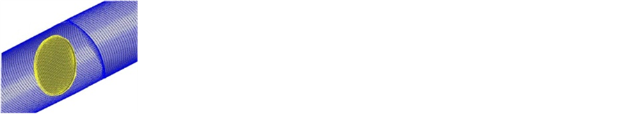

Figure 2. Grid system for simulating dynamic flat-plate flows (hybrid grid zone).
where ρ is the fluid density, u is the flow velocity vector, ug is the grid velocity of the moving mesh, Γ is the diffu- sion coefficient, Sf is the source term of f.
In order to satisfy the grid conservation law [18] the volume time derivative of the control volume is com- puted from
 (2)
(2)
3.2. Structure Dynamic Equation
The valve rotation can be described by the relationship,
 (3)
(3)
To obtain the flow field, the valve-closing process can be divided into incremental time steps. In each step, the blood pressure and the friction force computed from the previous time step is integrated over the leaflet surface to compute the moment due to the pressure and shear stress. The computational process shows in Figure 4. For fluid solver, a commercial CFD package, Fluent, is employed. The above described method was programmed as a user- defined function in Fluent. And Fluent-subroutine “Dy- namic Grid” was used for computational domain re- meshing.
The motion of the solid-body can be specified as a UDF code. The valve rotation Equation (3) can be de- scribed by the relationship,

 (4)
(4)
Equation (4) is a linear function so we increment the “adaptive time step method” in the UDF code as show in Figure 4. Using the adaptive time step method lets the determined pitch moment the same as in fluid and struc- ture solver.
3.3. Numerical Method
A pressure based finite volume method was used to solve the Equation (1). The contributions from the transient, total flux and source term in Equation (1) are assembled as flows. For each control volume the convection contri- butions from the adjacent volume as given by Equation (2) are summed and with the diffusion contributions and source contributions are substituted into Equation (1) to yield a system of equation of the from
 (5)
(5)

Figure 3. Numerical boundary condition enforcement.

Figure 4. FSI procedures.
which may be solved for the dependent variable f using any suitable solver.
The pressure correction equation is derived from the continuity equation where the velocity terms are substi- tuted with the velocity correction terms [19], given by


 (6)
(6)
where the “start” velocities u and v are the guessed ve- locities at the previous iteration. Integrating the continu- ity equation over an arbitrary control volume and apply- ing Green’s first theorem gives
 (7)
(7)
On application of the geometric conservation law [18]
 (8)
(8)
Using the corrected pressures by Equation (6) the ve- locity corrections are calculated and hence the corrected velocity is calculated and applied to the equation for convective mass flux and rearranging gives the system of equations which for the control volume surrounding node P may be expressed as
 (9)
(9)
Equation (9) may be solved using any suitable solver with the resulting solution used to update the variables in Equation (1).
3.4. Turbulent Model
Numerical and experimental results show that the time averaged Reynolds number in arteries is not high (300 - 500); however, when the waveform is up to peak value, Remax is near 2000 - 2300. Thus, the flow may become turbulent and hence a modified version of the Low- Reynolds-Number (LRN) k-ω model of Wilcox (1998) was selected [20].
4. Boundary Conditions
For the present pulsatile flow simulation, a prescribed inflow volume flowrate history is specified at the inflow plane. This aortic volume flow rate waveform, as shown in Figure 5, is adopted from an in-vitro experiment car- ried out by Simon et al. [21]. The present incompressible flow simulation requires a given velocity distribution be specified at the entrance plane. This velocity profile is unknown in advance although the volume flow rate is given. It is assumed in the present simulations that fully- developed pulsatile inflow is established in block I. For all the subsequent unsteady simulations, the inflow ve- locity distribution is calculated in a sub-iteration manner over block I before marching to the next time step. At each instant, a fully-developed parabolic laminar pipe flow velocity distribution corresponding to the specified volume flow rate is taken as the initial guess. Periodic boundary condition is enforced over the inflow and out- flow planes of block I during the sub-iterated pseudo time-marching until certain convergence criterion is sat- isfied.
Fully-coupled fluid/structure interaction is carried out by integrating together the fluid and structure equations. Since the volume flowrate is given, the occluder motion will be determined as a result interacted with the passing pulsatile flow. How would be the maximum opening angle reached for the occluder in heart systole is deter- mined by the specified inflow volume flowrate condition. In order to make the interaction simulation tractable, the impact dynamic modeling is not attempted presently. The closure criterion, therefore, is set by neglecting the asso- ciated occluder rebounding that might occur in the real valve flow.
5. Results and Discussion
5.1. Regurgitant Flow in the Diastolic Phase
Regurgitation in the diastolic phase represents a critical flow condition associated with many valve design con- siderations. Hemolysis and cavitation inception are two serious problems found with the regurgitant flow for mechanical heart valves. The high-speed jet emanating from the tiny clearance between valve edge and housing rim constitutes a high-shear and low-pressure flow char- acteristic which is prone to cavitation inception. The burst of the cavitation bubbles is very detrimental to blood cells and the valve structure as well. Experimental investigation of this regurgitant flow is difficult to per- form and CFD analysis becomes the alternative re- searchers are interested in. It was argued that the dimen- sion disparity, namely, the clearance size is of orders of magnitude smaller than the occluder diameter, allows

Figure 5. The aortic waveform generated by an in-vitro flow loop [21].
clearance flow be treated as a local phenomenon. The interaction with the much larger transvalvular main stream is assumed weak so almost all the investigations, to the author’s knowledge, were conducted based on a local viewpoint only. The boundary conditions specified on the two sides across the occluder are quiescent flows with given steady or transient pressure differential. The occluder was assumed either stationary or moving with a prescribed closing velocity. This regurgitant valve flow is herein revisited using the fully coupled FSI code. The appropriateness of taking regurgitant flow as of local and quasi-steady nature is re-evaluated.
There are 4 instants that are taken over the diastolic phase of the volume flow rate trace, representing differ- ent stages of the regurgitant flow. Two observation planes are selected to explore the regurgitant flow details. The first cross-sectional plane A-A is taken one channel height upstream of the occluder. The second plane, B-B, however, is defined in the clearance gap close to the jet exit. Steady-state simulation is carried out using the last instant (t = 800 ms) volume flowrate as the inflow condi- tion. The axial velocity distributions obtained for all in- stants, either simulated using unsteady or steady flow assumptions, show almost identical profiles at the B-B cross sectional plane, as illustrated in Figure 6. This im- plies that in the clearance gap, indeed, flow properties are local and quasi-steady. However, away from the jet exit, for example, at the downstream A-A plane, unsteady and quasi-steady simulations yield completely different re- sults.
Shown in Figure 7 is the axial velocity distribution. Similarity is found among the solution group simulated using the unsteady, coupled fluid/structure solver. Sharp contrast, however, exists between results computed under quasi-steady and unsteady assumptions. Intuitively it would be reasonable to expect that the unsteady result obtained at the late valve closure instant (t = 800 ms)

Figure 6. Compression of regurgitant axial velocity of pul- satile and steady flows in the clearance B-B plane.


Figure 7. Compression of regurgitant axial velocity of pul- satile and steady flows (X = −H, t = 340, 400, 500, and 800 ms).
would agree more with the quasi-steady result because the transient induced by valve closing should largely diminish or die out then. This physical intuition is proved to be wrong in Figure 8 using velocity vector plots. It is seen that the vortices obtained by the coupled fluid/ structure simulations encompass completely different fun- damental structures, suggesting that the flow characteris- tics before valve closure is essential.
Note that the quasi-steady simulation has a uniform, quiescent background flow to start with. In consequence, the clearance jets develop into a pair of symmetric, flat- tened vortices with high energy concentrated in the near wall regions. The wall shear stress which is important for predicting endothelial cell lesion is hence overestimated in the quasi-steady simulation.
Comparing to the quasi-steady result, the unsteady simulations show a more round and dominant vortex structure swirling around the occluder. All unsteady simulations, pertaining no matter to early or late instant in the diastolic phase, possess similar vortex structures. These vortices, in fact, are initiated long before the com- pletion of valve closure, attributed to the occluder closure motion. Right before the valve closure, a concentrated vortex core is produced in the upstream vicinity of the occluder trailing-edge. Lai et al. [14] also found a similar low-pressure vorticity zone occurring at similar place during valve closure, with vorticity strength dependent on the closure speed. When the occluder comes to a com- plete stop at the closure position, the clearance jet flows


 (a)
(a) (b)
(b) (c)
(c) (d)
(d)
Figure 8. Compression of regurgitant velocity vector plots of pulsatile and steady flows (X = −H, t = 340, 400, and 800 ms); (a) t = 340 ms; (b) t = 400 ms; (c) t = 800 ms; (d) Steady inflow.
develop and interact with this low-pressure vortex struc- ture. The upper jet energy was absorbed by this vortex, resulting in an even larger vortex resident next to the regurgitant flow side. The persistence of this lingering vortex diffuses the velocity shear originally contained in the wall jet regions. This explains why the unsteady simulation results have a mild velocity gradient distribu- tion which persists without decay over the entire diastolic phase.
This closure vortex and wall jet interaction phenome- non is newly found in the present fluid/structure interac- tion simulation. The previous concept that clearance flow characteristics can be taken as local and quasi-steady should be re-evaluated.
A viable leakage flow study cannot ignore the initial flow structure which is already in existence prior to the complete valve closure. The role of the trapped, lingering closure vortex should be included in the future regurgi- tant flow analysis. Otherwise, the structure of the valve leakage flow will be misinterpreted and the clinical im- plication could be wrongly overestimated.
5.2. Blood Cell Damage Evaluation
The results expected from a cardiovascular CFD analysis are not limited only to the flowfield investigations. More importantly, it needs an evaluation criterion to judge if the design is acceptable as considered from a broader blood cell damage or activation perspective. Researches [22-25] found that both shear stress and exposure time are important factors for accounting the breakdown of red blood cell membrane, which would cause protein hemoglobin to be released into the surrounding plasma. Although there are some disagreements existing in the calibration of the parameters involved in the empirical rule.
A general consensus is reached in controlled experi- ments that the ratio of damaged hemoglobin content to the total hemoglobin content can be expressed by a power law (proposed by Giersiepen et al. [9]):
 (10)
(10)
In the present CFD simulation a cumulative blood cell damage assumption is adopted. The hemolysis index HI is therefore defined using the following integral estimate [10],
 (11)
(11)
Cells are taken as passive markers carried by the stream. Lagrangian tracking is employed to define the instantaneous cell position and hence the stress experi- enced at the instant of observation. In tracking the parti- cles, residence time can also be obtained by adding up the time steps a particle has traveled since released from the inlet until discharged out of the exit. Longer resi- dence time usually correlates with higher potential of blood damage and thrombogenesis.
The inflow and exit planes for evaluating blood trauma are selected to be located at X = −10H and 10H, respec- tively. There are totally 40 particles that are released from the inlet plane and the accumulated HI values asso- ciated with each particle path line. Large HI values are found in general for particles drifted through the high- shear regions.
Since regurgitant flow is of particular significance to blood trauma, particle tracers are also released at the re- gurgitant phase. The results are shown in Figure 9. The regurgitated particles are squeezed through the upper and lower clearance gaps and the pathlines are greatly influ- enced by the vortex motion on the two sides of the leaflet. The vortex entrainment effect is best seen around t = 500 ms, and all particles leave the closure vortices eventually, as seen from the snapshot presented corresponding to t = 800 ms. During the particle traveling period the closure vortices do not change too much in their strength and position (see Figure 8), working as a cleaner to wash out the particles trapped in the leeward vicinity of the leaflet.
6. Conclusions
A fully-coupled fluid/structure interaction solver is de- veloped to simulate the transvalvuar flow passing over a tilting-disc prosthesis valve. Numerical simulation of a flat-plate occluder in an infinite straight duct is then conducted to explore the flowfield as interacted by an immersed moving occluder.
A pulsatile aortic volume flowrate history obtained from in-vitro test is specified as the inflow boundary condition. The resultant occluder motion is solved and the pitching moment trajectory shows a hysteresis loop when plotted against the opening angle, indicating dif- ferent transient dynamics is involved in the valve open- ing and closure phases. Flowfield details are disclosed using turbulent intensity, velocity, streamline, and vortic- ity snapshots corresponding to various instants of a pul- satile cycle. Complex vortex structures are found in the valve opening and closure phases. It is found in the pre- sent fully-coupled fluid/structure simulation that the vor-


Figure 9. Particle tracers in flow regurgitation, (unsteady simulation; 40 particles and released from cross sectional plane located at X/H = 1).
tices generated in the valve closure and regurgitant pe- riod encompass important mechanism which was over- looked in the past. During valve closure, the swing of the leaflet in the decelerated background stream generates different vortices around the two sides of the occluder. A low-pressure vortex core is further induced on the back side around the trailing-edge when leaflet is fully closed. This closure vortex is trapped around the occluder while interacting with the regurgitant jet flow. Contrary to the unsteady results, symmetric flattened vortex pair is ob- served in the quasi-steady simulation of the regurgitant flow, and the shear stress is overestimated. In summary, it is concluded that only fully-coupled fluid/structure si- mulation can yield correct description of a pulsatile transvalvular flow, in particular for analyzing the regur- gitant flow in the diastolic phase.
References
- 1. G. J. Cheon and K. B. Chandran, “Dynamic Behavior Analysis of Mechanical Monoleaflet Heart Valve Pros theses in the Opening Phase,” Journal of Biomechanical Engineering, Vol. 115, No. 4A, 1993, pp. 389-395. doi:10.1115/1.2895502
- 2. V. Kini, C. Bachmann, A. Fontaine, S. Deutsch and J. M. Tarbell, “Flow Visualization in Mechanical Heart Valves: Occluder Rebound and Cavitation Potential,” Annals of Biomedical Engineering, Vol. 28, No. 4, 2000, pp. 431-441. doi:10.1114/1.281
- 3. D. Bluestein, E. Rambod and M. Gharib, “Vortex Shed ding as a Mechanism for Free Emboli Formation in Mechanical Heart Valves,” Journal of Biomechanical Engineering, Vol. 122, No. 2, 2000, pp. 125-134. doi:10.1115/1.429634
- 4. L. F. Hiratzke, N. T. Kouchoukos, G. L. Grunkemeier, D. C. Miller, H. E. Scully and A. S. Wechlser, “Outlet Strut Fracture of the Bjork-Shiley 60° Convexo-Concave Valve: Current Information and Recommendations for Patient Care,” Journal of the American College of Cardiology, Vol. 11, No. 5, 1998, pp. 1130-1137.
- 5. T. A. Odell, J. Durandt, D. M. Shama and S. Vythilingum, “Spontaneous Embolization of a St. Jude Prosthetic Mitral Valve Leaflet,” Annals of Thoracic Surgery, Vol. 39, No. 6, 1985, pp. 569-572. doi:10.1016/S0003-4975(10)62003-6
- 6. A. A. Mikhail, R. Ellis and S. Johnson, “Eighteen-Year Evolution from the Lillehei-Kaster Valve to the Omni Design,” Annals of Thoracic Surgery, Vol. 48, No. 3, 1989, pp. 561-564. doi:10.1016/0003-4975(89)90641-3
- 7. C. W. Lillehei, A. Nakib, R. L. Kaster, B. R. Kalke and J. R. Rees, “The Origin and Development of Three New Mechanical Valve Designs: Thoroidal Disc, Pivoting Disc, and Rigid Bileaflet Cardiac Prostheses,” Annals of Thoracic Surgery, Vol. 48, No. 3, 1989, pp. S35-S37. doi:10.1016/0003-4975(89)90630-9
- 8. R. Paul, J. Apel, S. Klaus, F. Schügner, P. Schwindke and H. Reul, “Shear Stress Related Blood Damage in Laminar Couette Flow,” Artificial Organs, Vol. 27, No. 6, 2003, pp. 517-529. doi:10.1046/j.1525-1594.2003.07103.x
- 9. M. Giersiepen, L. J. Wurzinger, R. Opitz and H. Reul, “Estimation of Shear Stress-Related Blood Damage in Heart Valve Prostheses—In Vitro Comparison of 25 Aortic Valves,” The International Journal of Artificial Organs, Vol. 13, No. 5, 1990, pp. 300-306.
- 10. L. J. Wurzinger, R. Opitz and H. Eckstein, “Mechanical Bloodtrauma: An Overview,” Angeiologie, Vol. 38, No. 3, 1986, pp. 81-97.
- 11. A. P. Yoganathan, Z. He and S. C. Jones, “Fluid Mechanics of Heart Valve,” Annual Review of Biomedical Engineering, Vol. 6, 2004, pp. 331-362. doi:10.1146/annurev.bioeng.6.040803.140111
- 12. T. K. Hung and G. B. Schuessler, “Computational Analysis as an Aid to the Design of Heart Valves,” Chemical Engineering Progress Symposium Series, Vol. 10, No. 9, 1971, pp. 8-17.
- 13. A. D. Au and H. S. Greenfield, “Computer Graphics Analysis of Stresses in Blood Flow through a Prosthetic Heart Valve,” Computers in Biology and Medicine, Vol. 4, No. 3-4, 1975, pp. 279-291. doi:10.1016/0010-4825(75)90039-6
- 14. C. S. Peskin, “Flow Patterns around Heart Valves: A Numerical Method,” Journal of Computational Physics, Vol. 10, No. 2, 1972, pp. 252-271. doi:10.1016/0021-9991(72)90065-4
- 15. J. de Hart, G. W. M. Peters, P. J. G. Schreurs and F. P. T. Baaijens, “A Two-Dimensional Fluid-Structure Interaction Model of the Aortic Value,” Journal of Biomechanics, Vol. 33, No. 9, 2000, pp. 1079-1088. doi:10.1016/S0021-9290(00)00068-3
- 16. M. J. King, T. David and J. Fisher, “Three-Dimensional Study of the Effect of Two Leaflet Opening Angles on the Time-Dependent Flow Througha Bileaflet Mechanical Heart Valve,” Medical Engineering & Physics, Vol. 19, No. 5, 1997, pp. 235-241. doi:10.1016/S1350-4533(96)00066-5
- 17. C. S. Peskin and D. M. McQueen, “Modeling Prosthetic Heart Valves for Numerical Analysis of Blood Flow through the Heart,” Journal of Computational Physics, Vol. 37, No. 1, 1980, pp. 113-132. doi:10.1016/0021-9991(80)90007-8
- 18. M. Vinokur, “An Analysis of Finite-Difference and Finite-Volume Formulations of Conservation Laws,” Journal of Computational Physics, Vol. 81, No. 1, 1989, pp. 1-52. doi:10.1016/0021-9991(89)90063-6
- 19. S. V. Patankar, “Numerical Heat Transfer and Fluid Flow,” Hemisphere, Ch. 6, 1980.
- 20. C. Kleinstreuer and Z. Zhang, “Laminar-to-Turbulent Fluid-Particle Flows in Human Airway Model,” International Journal of Multiphase Flow, Vol. 29, No. 2, 2003, pp. 271-289. doi:10.1016/S0301-9322(02)00131-3
- 21. H. L. Leo, H. Simon, J. Carberry, S. C. Lee and A. Yoga Nathan, “A Comparison of Flow Field Structures of Two Tri-Leaflet Polymeric Heart Valves,” Annals of Biomedical Engineering, Vol. 33, No. 4, 2005, pp. 429-443. doi:10.1007/s10439-005-2498-z
- 22. M. Grigioni, C. Daniele and U. Morbiducci, et al., “The Power-Law Mathematical Model for Blood Damage Prediction: Analytical Developments and Physical Inconsistencies,” Artificial Organs, Vol. 28, No. 5, 2004, pp. 467-475. doi:10.1111/j.1525-1594.2004.00015.x
- 23. D. F. Su and C. Y. Miao, “Blood Pressure Variability and Organ Damage,” Clinical and Experimental Pharmacology and Physiology, Vol. 28, No. 9, 2001, pp. 709-715. doi:10.1046/j.1440-1681.2001.03508.x
- 24. R. Paul, J. Apel, S. Klaus, F. Schagner, P. Schwindke and H. Reul, “Shear Stress Related Blood Damage in Laminar Couette Flow,” Artificial Organs, Vol. 27, No. 6, 2003, pp. 517-529. doi:10.1046/j.1525-1594.2003.07103.x
- 25. D. Arora, M. Behr and M. Pasquali, “A Tensor-Based Measure for Estimating Blood Damage,” Artificial Organs, Vol. 28, No. 11, 2004, pp. 1002-1015. doi:10.1111/j.1525-1594.2004.00072.x
*Corresponding author.