International Journal of Geosciences
Vol.05 No.09(2014), Article ID:48793,25 pages
10.4236/ijg.2014.59078
Integrated Geophysical, Remote Sensing and GIS Studies for Groundwater Assessment, Abu Zenima Area, West Sinai, Egypt
Mohamed H. Khalil1, Khalid S. Ahmed1, Alaa Eldin H. Elnahry2, Alaa N. Hasan2*
1Geophysics Department, Faculty of Science, Cairo University, Giza, Egypt
2Scientific Training and Continuous Research Division, National Authority for Remote Sensing and Space Sciences, Cairo, Egypt
Email: *alaa_nayef@hotmail.com
Copyright © 2014 by authors and Scientific Research Publishing Inc.
This work is licensed under the Creative Commons Attribution International License (CC BY).
http://creativecommons.org/licenses/by/4.0/


Received 29 April 2014; revised 21 May 2014; accepted 15 June 2014

ABSTRACT
The integration between advanced techniques for groundwater exploration is necessary to protect and to manage the vital resources. Enhanced Thematic Mapper Landsat (ETM+) images, a geographic information system (GIS), hydrological modeling and direct current (DC) resistivity geoelectrical techniques were used in integrated manner to identify the groundwater potentialities in the study area. The study area is approximately 1195 km2, located at the western portion of south Sinai. From the results of the eight thematic layers as input to GIS model, the suitable locations for dams could be estimated in the two main drainage basins Matulla and Tayiba.
Keywords:
Groundwater, Electrical Method, GIS, Remote Sensing

1. Introduction
Nowadays establishing new urban communities and expanding the existing ones have become one of the highest priorities for the decision makers in Egypt. The goal of this strategy is basically to reduce the dense population around the Nile valley. Abu Zenima area is located at the western coast of the Sinai Peninsula (Figure 1). It had seen potentially grown in connection with development projects, new urbanization, oil exploration, land reclamation, and tourism. Systematic planning and managing for groundwater exploration using modern techniques is implemented for the proper utilization, protection and management of this vital resource. Enhanced Thematic Mapper Landsat (ETM+) images, geographic information system (GIS), hydrological modeling and direct
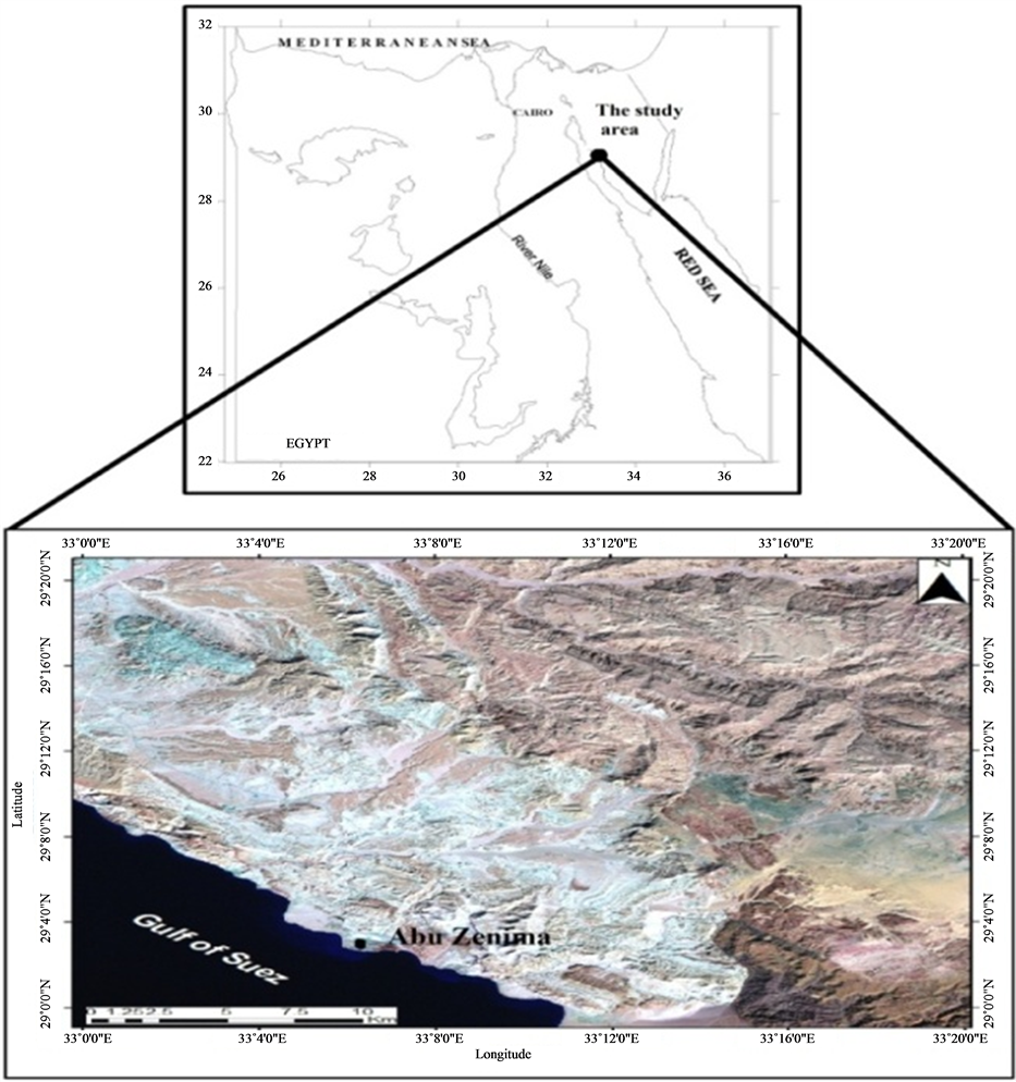
Figure 1. Location map of the study area, western coast of the Sinai Peninsula.
current (DC) resistivity geoelectrical techniques were integrated to achieve this approach.
Remotely sensed data were used to delineate the alluvial active channels, which were integrated with morphometric parameters extracted from digital elevation models (DEM) into geographical information systems (GIS) to construct a hydrological model that provided estimates about the amount of surface runoff, precipitation and the net recharge of groundwater aquifer.
A direct current (DC) resistivity electrical technique was applied in Abu Zenima area to determine and evaluate the main aquifer in this area. For that concern, twenty two Schlumberger vertical electrical soundings (VES) with maximum AB/2 = 3000 m were conducted. The interpretation of the one-dimensional (1-D) inversion of the acquired resistivity data were implemented for mapping the fresh to slightly brackish water aquifer. Subsurface lithological information and the depth to the top of ground water table (obtained from the existing boreholes) (Khalil, 2006) [1] are used to calibrate the results of the resistivity data inversion.
This research discussed how the integration between the geoelectrical parameters and hydrological data, could be used to determine the appropriate locations of dams construction.
Extensive work had been carried out by the Egyptian government to restore the groundwater quality in the densely populated and/or highly developed areas such as Abu Zenima. A number of previous geological, hydrological, and geophysical studies were carried out in Abu Zenima by many researchers (Shata, 1956 [2] ; Butzer, 1960 [3] ; Geofizika, 1963 [4] [5] ; El-Kiki, 1965 [6] ; Youssef et al., 1966 [7] ; Ettinger et al., 1969 [8] ; Evenari et al., 1971 [9] ; Tewfic, 1975 [10] ; Bishay, 1979 [11] ; Shata, 1979 [12] ; Hammad, 1980 [13] ; Saad et al., 1980 [14] ; El-Ayouty et al., 1984 [15] ; El-Refaei, 1984 [16] ; El-Shazly et al., 1985 [17] ; Klitzsch and Schrank, 1987 [18] ; El-Refaei, 1992 [19] ; Shata et al., 1992 [20] ; Kusky et al., 1994 [21] ; Abd El Rahman, 2001 [22] ; Masoud and Koike, 2005 [23] ; Khalil, 2006 [1] ; Mills and Shata, 2009 [24] ; Elewa and Atef, 2011 [25] ).
2. Geological Setting
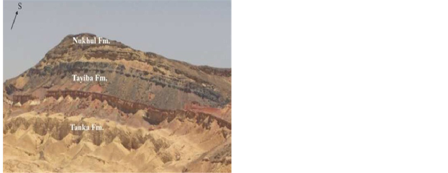
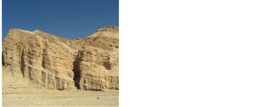
The investigated area is located at the western portion of south Sinai between latitudes 29˚00'N and 29˚20'N and longitudes 33˚00'E and 33˚20'E. It is bounded from the west by the Gulf of Suez and the Suez Canal and from the east by Gulf ofAqaba, while bordered by the Mediterranean Sea from thenorth and Red Sea from the south (Figure 1). The foreshore plain in Abu Zenima area is covered with Plio-Pleistocene and Recent unconsolidated sediments and dominated by mobile sands. Along the Gulf of Suez, the foreshore plain is characterized by the presence of alluvial fans (El-Refaei, 1992) [19] . Figure 2 indicates a wide range of geological time scales ranging from Pre-Cambrian to Quaternary. The Quaternary deposits are differentiated into upper and lower regions of recent and Pleistocene deposits, respectively, while the late pre-rift stratigraphy consists of a carbonate- dominated Eocene succession (Thebes, Darat, Khababa and Tanka Formations) (Jackson et al., 2002) [26] . A late Oligocene to early Miocene syn-rift strata unconformably overlies these pre-rift units. The Abu Zenima and Nukhul Formations are thought to have been deposited in fluvial to shallow marine environments during a slow subsidence rift-initiation phase where sedimentation took place with subsidence (Gawthorpe et al., 2003) [27] . Overlying the Nukhul Formation are deep marine deposits of the rift climax lower Rudeis Formation (Figures 3(a)-(d)).
The pattern of faults in the central dip province of the Gulf of Suez controls the structure of the main geological units. It can be divided into two major families; the first pattern is longitudinally parallel to the axis of the rift created in an extensional regime during the Neogene, and the second pattern consists of transverse faults with N-S to NE-SW dominant trends that inherited passive discontinuities in the Precambrian basement rock (Colletta et al., 1988) [28] .
Eight oil, exploration and water boreholes were drilled in the study area; three of them (I, II and III) are deep—up to 500 m (GUPCO 1960, 1975) [29] , whereas the other five (1 through 5) are shallower—up to 70 m (Egyptian Desert Research Institute 2004) [30] (Figure 4).
3. Geoelectrical Measurements
The study area extends 32.37 km in width by 36.94 km in length .A total number of 22 Schlumberger Vertical Electrical Soundings (VES) were conducted in Abu Zenima area with maximum current electrode half-spacing (AB/2) of 3000 meters (Figure 4). All VES were well distributed taking into consideration the complex tectonic system of the study area. Some VES were conducted very close to available water wells (Egyptian Desert Research Institute, 2004) [30] to correlate the well data with the resultant resistivity data.
Resistivity measurements were carried out using a digital signal-enhancement resistivity-meter (GISCO USA, ABEM-TERRAMETER, SAS 4000), which permitted high accuracy due to its advanced technical specifications (24 bit BITSTREAM A/D conversion, receiver of up to 140 dB dynamic range plus 64 dB automatic gain control, 10 MegaOhm input impedance, 30 nV resolution, transmitter 1 - 1000 mA, 400 V maximum output voltage and 100 W maximum output power (Figure 5). A DC current was injected into the earth via two current electrodes and the potential difference between the two electrodes was measured via two potential electrodes. Apparent resistivity was then calculated by multiplying the geometric factor of the used Schlumberger array by the measured resistance value. The resistivity data was measured every sixth of a logarithmic decade to ensure interpretation accuracy.
Field data was interpreted through three steps: a) smoothing of the field data curve during data acquisition; b) preparing an initial model depending on the geological background as well as the previously drilled boreholes;
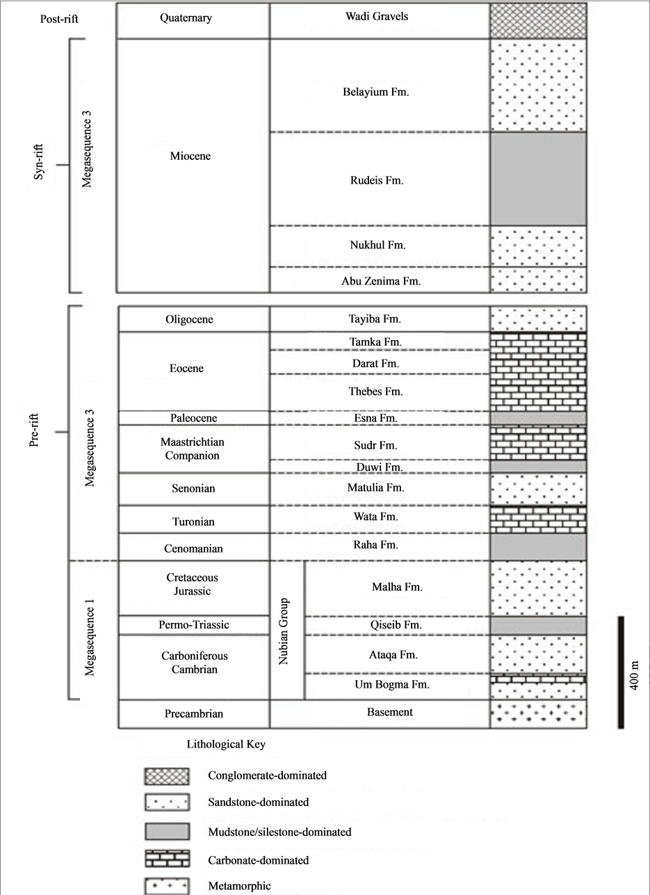
Figure 2. Subsurface stratigraphic section in the study area (After Jackson et al., 2002).
 (a) (b)
 (c) (d)
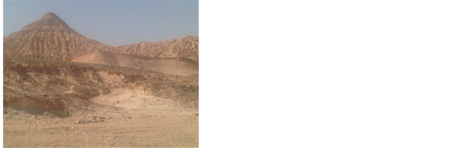
Figure 3. (a) The classical section of Abu Zenima formations; (b) Daraat Formation, lower Thal valley; (c) A typical section of Nukhul/Tayiba formations; (d) Gabal Matulla.
and c) introducing the initial models into the Van Der Velpen (1988) [31] software (Khalil, 2006; Khalil, 2012; Khalil, 2013) [1] [32] [33] . Iterations were carried out to reach the best fit between the smoothed field curve and the calculated one. The root mean square (RMS) errors of the resulted models ranged from 3.5% to 8.4%. Figure 6 illustrated two samples of the conducted data after the final interpretation processes (VES’s 16, 17) correlated with the some corresponding adjacent boreholes (wells 5 and III).
4. Data Analysis and Interpretation
The interpreted VES stations were used to produce four geoelectric cross sections (Figure 7). Data from oil, exploration and/or water wells were integrated in these sections. Faults shown in these cross-sections were confirmed from geological studies performed in the study area (Egyptian Desert Research Institute, 2004) [30] .
Four subsurface layers were recognized in the geoelectric cross sections from top to bottom as follows:
1) A surface layer was characterized by variable apparent resistivities(70 - 955 Ohm∙m) and correspond to Plio-Pleistocene and Recent surficial deposits; silt, sand, and gravel sediments. Variations in the resistivity values of this layer could be attributed to two main reasons: areal variations in the grain size distribution and variation in the gravel-sand-silt-clay ratios. The thickness of this layer ranges between 1 and 8 m.
2) A second layer represents the fresh to slightly brackish water bearing formation. The resistivities of this layer ranges between 36 and 71 Ohm∙m, corresponding to Plio-Pleistocene and Recent silt and sandstone. The thickness of this layer ranges between 10 and 66 m.
3) A third layer is characterized by very low resistivities (2.2 - 5 Ohm∙m), it corresponding to Miocene-eva- porite group (marl, gypsum, and anhydrite). The low resistivity values of this layer are due to the salt seawater intrusion as well as the dissolution of the Miocene-evaporite group. The top of this layer is considered to be
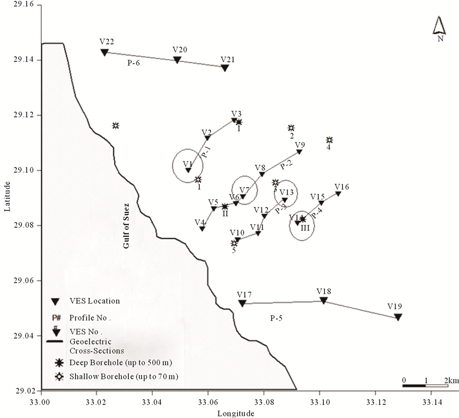
Figure 4. VES location map of the study area.
the bottom of the fresh to brackish water bearing layer (the freshwater floats over the denser more salt deeper water). The thickness of this layer ranged between 162 to 405 m.
4) A bottom layer was characterized by very low resistivities ranging between 3.1 - 3.8 Ohm∙m, corresponds probably to Miocene limestone.
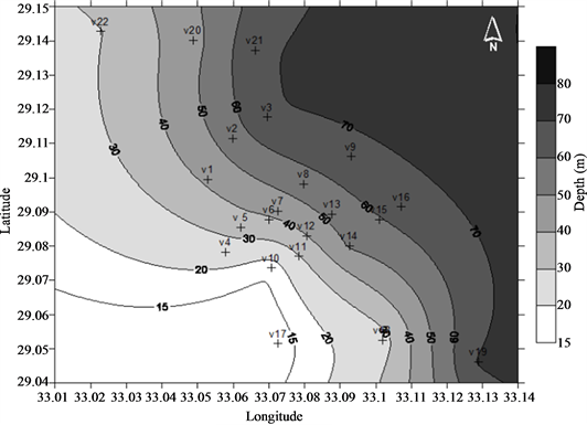
Figures 8(a)-(c) respectively illustrated the contour maps of the depth (m), thickness (m), and resistivity (Ohm∙m) of the fresh to slightly brackish subsurface aquifer in the study area. The thickness of the fresh to slightly brackish aquifer ranged from 10 and 66 m. The aquifer thickness increased toward the northeastern part of the study area. The aquifer has true resistivity range from 36 to 71 (Ohm∙m) with an increase toward the northeastern part.
5. Remote Sensing and GIS
The advent of remote sensing technology and geographical information system (GIS) tools opened new path in water resource interpretation. The most important potential application of GIS in hydrological modeling is the determination of geometric and topographic parameters from digital elevation model (DEM). The determination of these hydrological parameters has received much attention in the literature in recent years, as the automated use of data from digital elevation model, such as surface slope, channel length and flow direction, has become
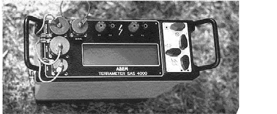
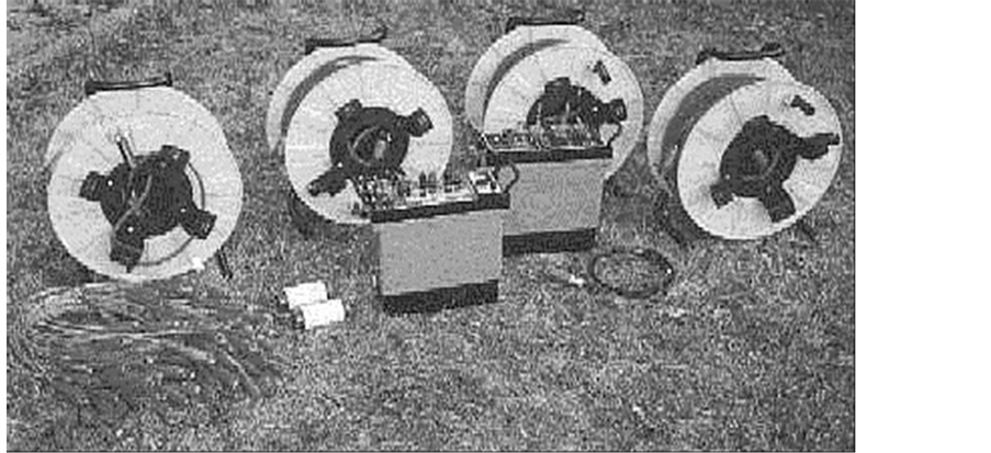
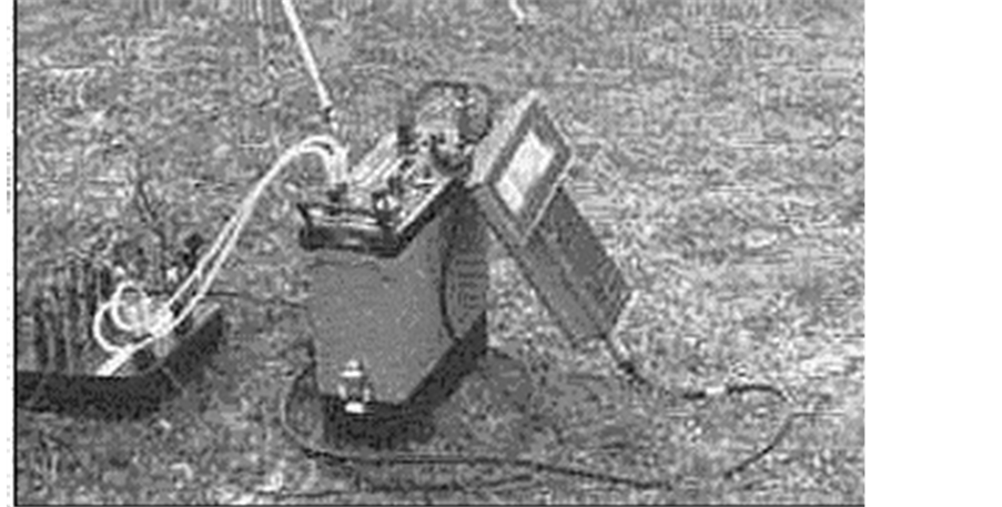
Figure 5. ABEM Resistivity meter with accessories.
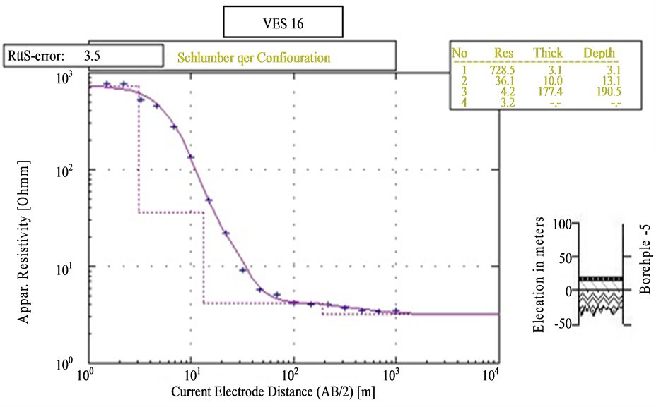
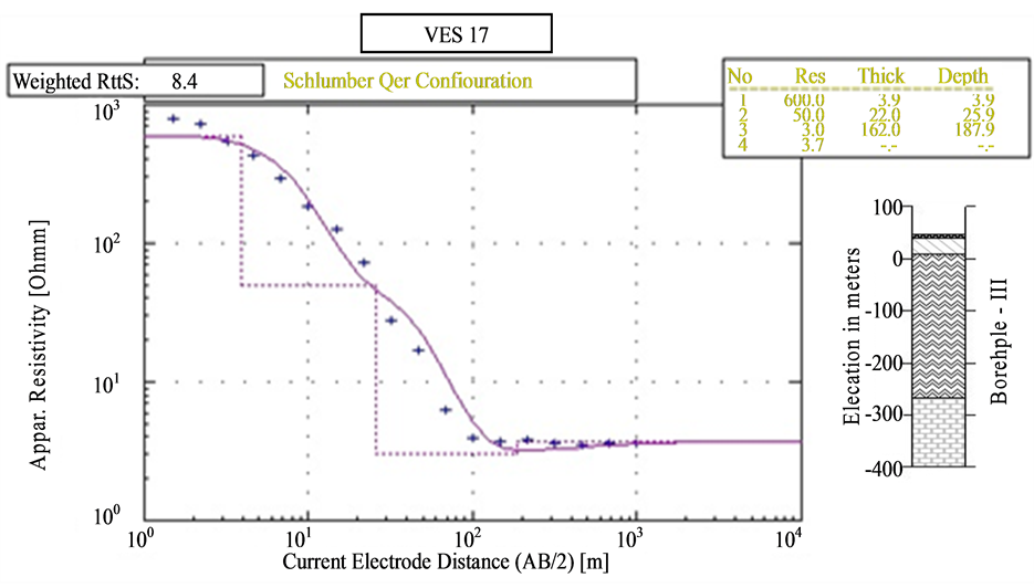
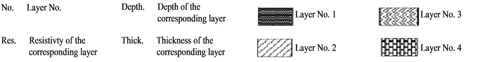
Figure 6. Correlation between the interpreted resistivity layers of the selected VES’s and the given borehole data.
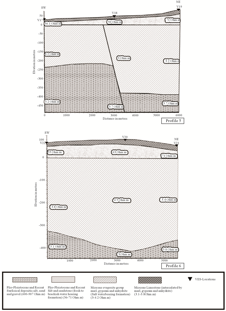
Figure 7. Geoelectric cross-sections of Profiles-5 and -6 in the study area.
 (a)
(a)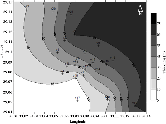 (b)
(b)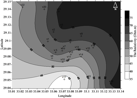 (c)
(c)
Figure 8. Three contour maps showing (a) the depth (m), (b) the thickness (m) and (c) the true resistivity (Ohm∙m) maps of the fresh water bearing layer, respectively.
widespread (Jenson and Dominque, 1988 [34] ; Moore et al., 1991 [35] ; Maidment, 1993 [36] ).
Using an elevation raster or digital elevation model (DEM) (Figure 9), it is possible to automatically delineate a drainage system and quantify the characteristics of the system. The Digital elevation model (DEM) was processed to automatically extract the drainage networks using the original D-8 algorithm embedded in ArcInfo software with some modifications in the filling of DEM step (El Bastawesy, 2005) [37] . This model required, first, that all the sinks (i.e. local depressions) of the DEM to be filled and raised in elevation to their neighbouring cells in order to ensure the flow continuity within the catchment to an outlet (Jenson and Dominique, 1988) [34] (Figure 10). After the DEM was filled, the flow direction of each cell into the lowest elevation cell of the surrounding eight cells was determined. Once the route of flow was determined for each cell in the DEM (Figure 11), it is possible to accumulate the number of upslope flow contributing cells (i.e. areas) and the flow paths of each cell (Figure 12). Then the output from flow direction was used as input to produce the output raster that delineates the drainage basins (El Bastawesy, 2005) [37] . The drainage lines were traced and compiled into four hydrographic basins using the available aerial photograph and DEM (Figure 9). The studied basins had down streams inside the study area (Figure 13). Afterward the stream order tool was applied by Strahler technique (Strahler, 1952) [38] to represent the order of each of the segments in a network (Figure 14) and (Figure 15).
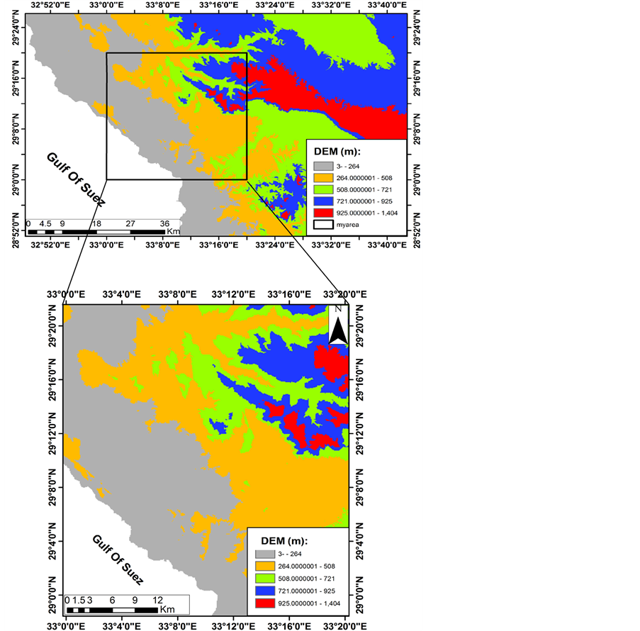
Figure 9. Digital Elevation Model (DEM) of the study area.

Figure 10. Fill DEM of study area.
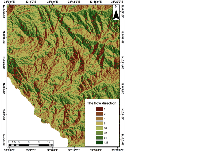
Figure 11. Flow direction map of the study area.
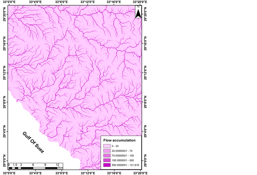
Figure 12. Flow accumulation map of the study area.
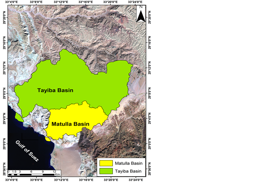
Figure 13. Studied basins of the study area.
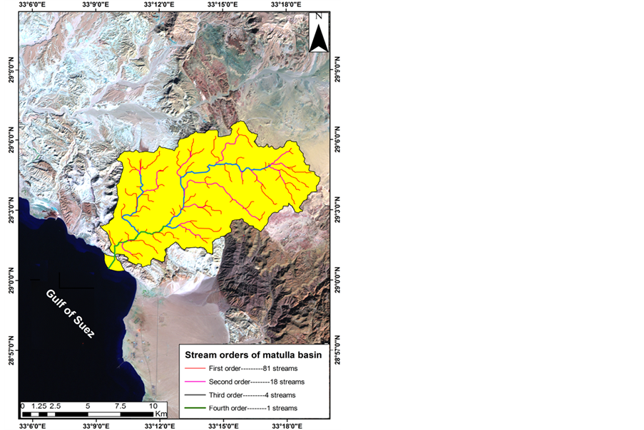
Figure 14. Stream order of Matulla basin.

Figure 15. Stream order of Tayiba basin.
6. Hydrological Budget of the Basins in the Study Area
Hydrographic parameters associated with the drainage basins of the study area are given in Table 1. However, the infiltration capabilities and groundwater potentiality for the rocks of the study area is given in Table 2.
7. Site Selection Model
A site selection model is a decision making tool for identifying locations in a landscape where multiple criteria overlap in geographic space (Wilson, 2008) [39] . The primary goal of this study is development a methodology to locate suitable locations for constructing dams and the secondary goal is to identify the factors which govern this selection. GIS program was used as a tool helps to attain this goal.
1) Conditions that govern the selection of the suitable locations for dams’ construction:
· Slope
Slopes help to identify the maximum rate of change in surface value over a specific distance and they are expressed in degrees or percentage (Anavberokhai, 2008) [40] . The slope map (Figure 16), was obtained from the DEM shows the slope variation in the study area. Slope steepness plays an important role in the selection of suitable locations for dams’ construction. Therefore a site with minimum topographical gradient will render best services for building dams. A gradient between 0.2% and 4% is perfect, but slopes up to 15% could also be used in worst cases (Ziadat et al., 2006) [41] .
· Earthquakes
Seismic activity is the study of the distribution of earthquakes and their characteristics within a particular region. The most important aspects of seismic activity are given by the geographic distribution of earthquakes` foci, their magnitude and their occurrence over time. The mechanisms and the damage produced by the earthquakes that affected this area, were studied by Dahy (2010) [42] . In Egypt, the earthquake activity has been observed in various regions. It is important to build dams on the site with low seismicity to protect the downstream lifeand property. Generally, strong ground shaking can result instability of the dam andstrength loss of foundations. (Seed et al., 1969 [43] ; Seed et al., 1975 [44] ; Jansen, 1988 [45] ; Castro et al., 1985 [46] ).
· Buildings and roads
In general, buildings haven’t to be located near dams because their sewage pipelines can affect the soil cohesion where dams are built. Also dams have to be away from roads where traffic can cause vibrations in dams’ bodies like earthquakes.
· Drainage network
The dams are preferred to be built on the main stream order where the most common point of collection of runoff.
2) The layer using in model
Drainage Network, Elevation, Slope, Buildings, Roads, Earthquakes and Faults were used as input data in model which were explained in Table 3. They governed the selection of the suitable locations for dams’ construction. They were explained in detail in paragraph 1.
3) Methodology
It will be built a suitability model with ArcGIS Spatial Analyst extension tools that finds suitable locations for

Table 1. Hydrographic parameters and GIS outputs for the study area drainage basins.
Table 2. Major exposed rocks in the study area according to their infiltration capabilities and groundwater potentiality.
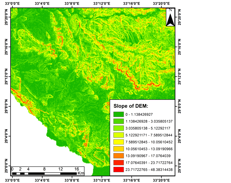
Figure 16. Slope for DEM of the study area.
Table 3. The layer using in model.
a dam’s construction. The steps to produce such a suitability model are outlined below:
1) Drainage Network, Elevation, Slope, Buildings, Roads, Earthquakes and Faults were used to design site selection model in Table 4 as input for model;
2) Deriving distance from recreation sites;
Euclidean distances were estimated to calculate the distance between every layer and surrounding grids. In other word, it must first be calculated the Euclidean (straight-line) distance from recreation sites. On the Distance to recreation sites layer, distances increase the farther you are from a recreation site (ESRI, 2011) [47] . Some samples of maps were shown in Figure 17, Figure 18.
Table 4. Weighted overlay model.
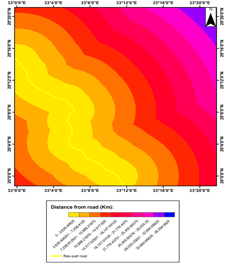
Figure 17. Distance from the road in the study area.
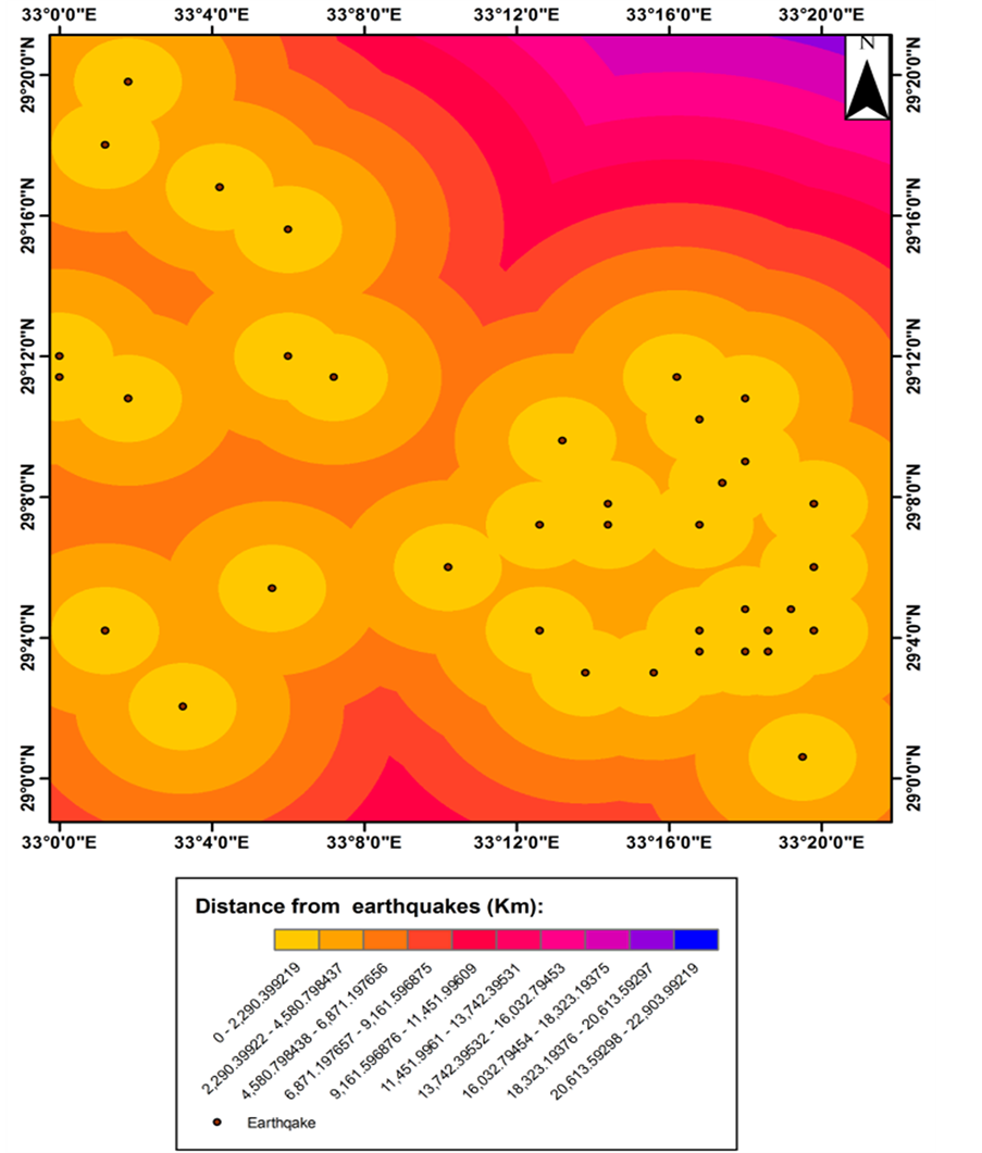
Figure 18. Distance from the earthquakes in the study area.
3) Reclassifying datasets
Deriving datasets, such as slope, is the first step when building a suitability model. Each cell in the study area now has a value for each input criteria (distance to Drainage Network, distance to Elevation, distance to Buildings, distance to Roads, distance to Earthquakes, distance to Faults, Slope). It needs to be combined the derived datasets so it can be created the suitability map that will identify the potential locations for the dams’ construction. However, it is not possible to combine them in their present form so the next step was to reclassify the previous maps where they were classified into a relative friction of 10 classes in order to have a common value. In the classified maps, the number “10” indicated good areas to construct dams while the number “1” indicated bad areas. For example, it is necessary to construct dams away from earthquakes to protect the downstream life and property so It will be reclassified the Distance to earthquakes layer, assigning a value of 10 to areas farthest from existing earthquakes (the most suitable locations), assigning a value of 1 to areas near earthquakes (the least suitable locations), and ranking the values in between linearly. By doing this, it will be determined which areas are near and which areas are far from earthquakes. Some samples of maps were shown in Figure 19, Figure 20.
4) Weighting and combining datasets
It is now ready to combine the reclassified datasets to find the most suitable dams construction. The values of the reclassified datasets have all been reclassified to a common measurement scale (more suitable cells have higher values) and weighted each according to its importance where it will be weighted all the inputs, assigning each a percentage of influence. The higher the percentage, the more influence a particular input will have in the suitability model (Table 4, Table 5).
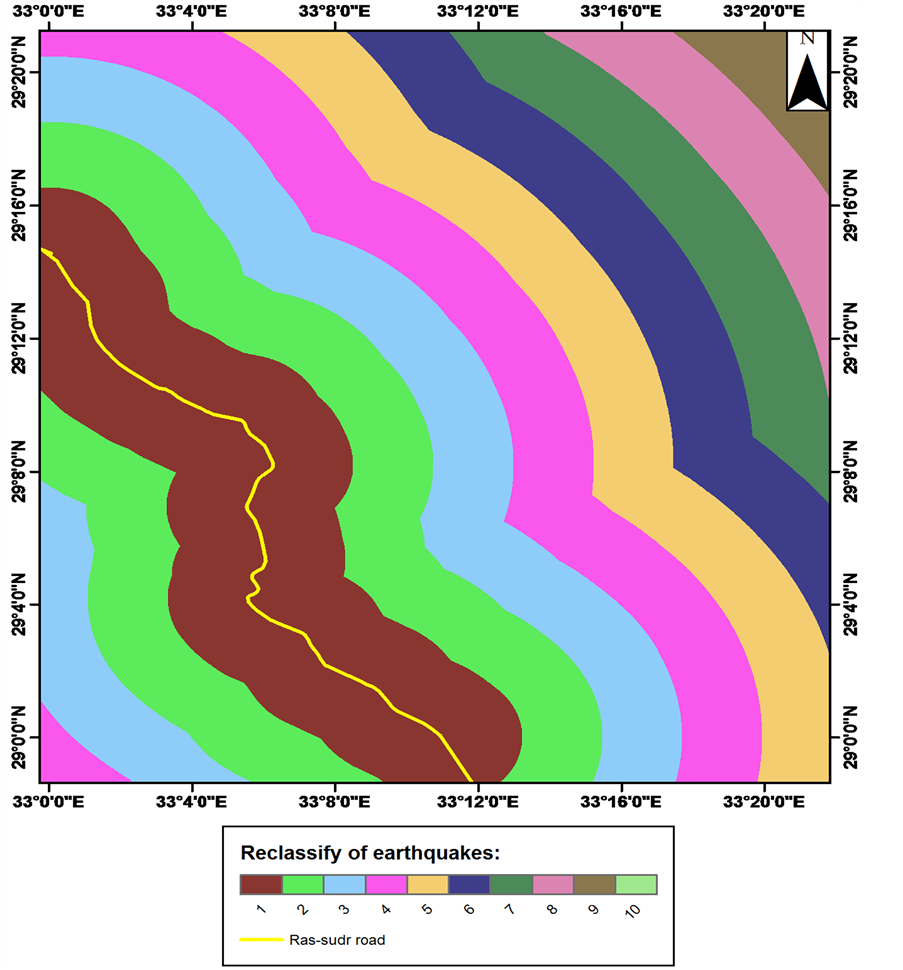
Figure 19. Reclassify for road of the study area.
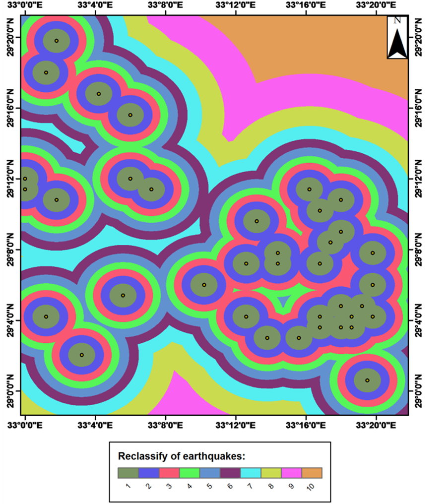
Figure 20. Reclassify for earthquakes in the study area.
Table 5. Intensity of importance.
5) Selecting optimal sites
Now each pixel has a value that indicates how suitable that location is for dams’ construction. Pixels with the value of 10 are most suitable, and pixels with the value of 0 are not suitable. Therefore, the optimal site location for dam construction has the value of 10. Another criteria for an optimal location is the size of the suitable area. A suitable location would include several pixels with value of 10 being connected. It will be used a conditional expression in the Con tool to extract only the optimal sites. It has been decided that those sites that are considered optimal must have a suitability value of 10 (the highest value in the suit areas output). In the conditional expression, all areas with a value of 10 will retain their original value (10). Areas with a value of less than 10 will be changed to No Data (ESRI, 2011) [46] (Figure 21). Then applying feature to points tool which creates a feature class containing points generated from the representative locations of input features (ESRI, 2011) [47] . Where the tool proposes several locations while the interpreter tries to find the optimum locations for construction dams where the highest amount of water (Figure 22). Flow chart showing the procedures to establish the site selection model for selecting the suitable locations for construction dams (Figure 23).
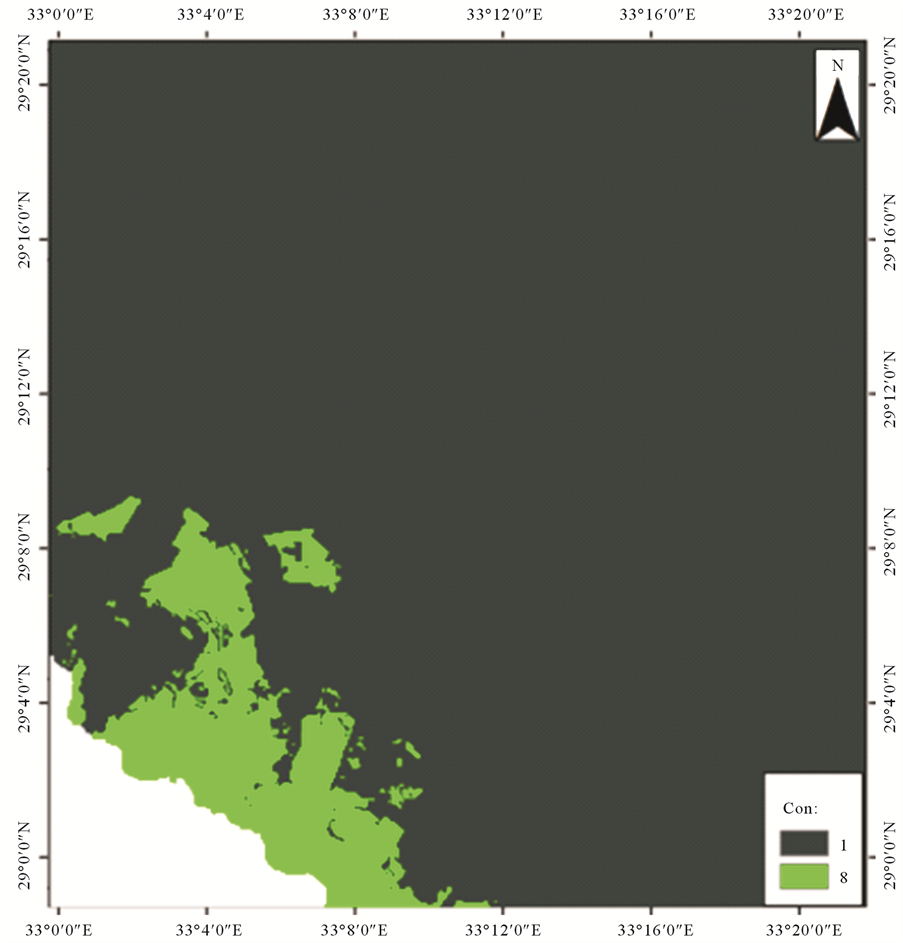
Figure 21. Con for the weighted overlay map.
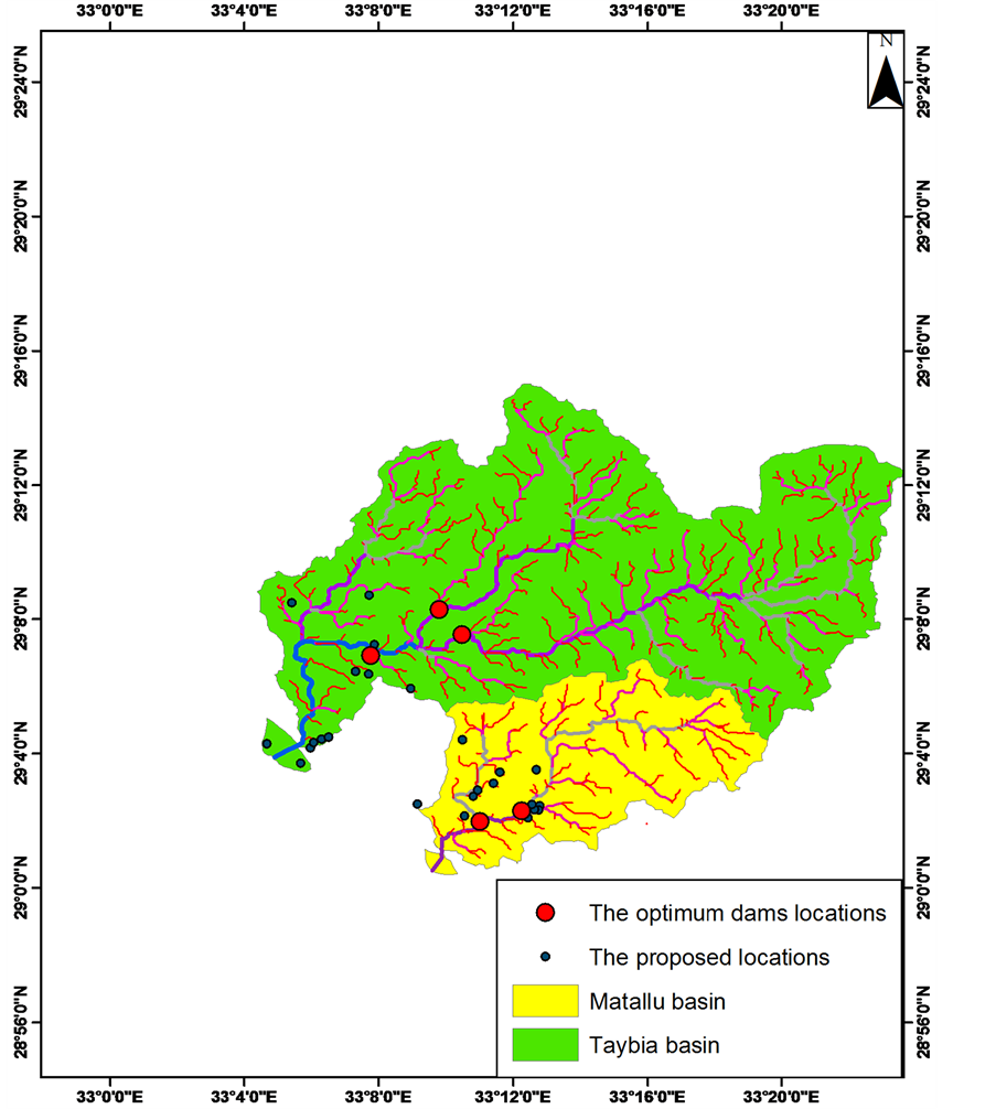
Figure 22. Drainage system in the study area, the minor points show the proposed locations from model and the major points show the optimum locations of dams by interpreter.
8. Conclusions
The integration between the geoelectrical parameters, hydrological data and geographic information systems (GIS), was a successful approach in the site selection process to identify the optimum locations for dam construction. Furthermore, the approach implemented was successful in estimation of the hydrological budget in the study area as it has facilitated the determination of the surface runoff, net groundwater recharge for each basin and consequently the exploitable groundwater storage in the aquifer. The results showed that the total runoff in the study area is 3,770,189 m3/year, the surface runoff is 2,165,077 m3/year, the net groundwater recharge is 1,605,112 m3/year and the time to peak discharge is 2956 min.
The results of the Vertical Electrical Sounding (VES) showed that the fresh aquifer has a thickness ranging
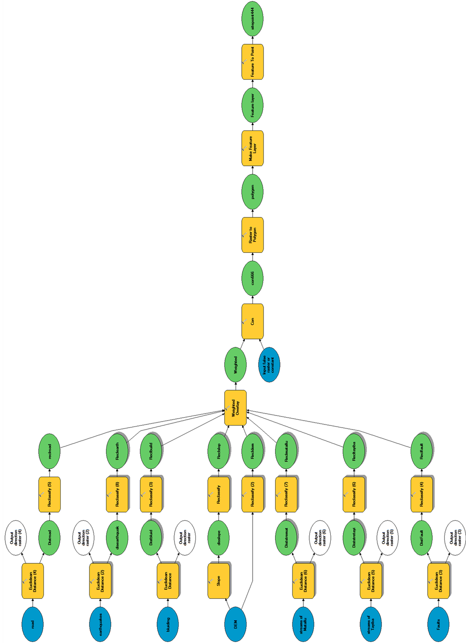
Figure 23. Flow chart of site selection model.
from 10 m to 66 m with resistivities ranging from 36 Ohm∙m to 71 Ohm∙m. This fresh-water aquifer floats over the denser, more saline, deeper water (resistivities 2.2 - 5 Ohm∙m). Moreover, it was evident that the southwestern part of the study area (downstream of Abu Zenima) represents the optimum location for the drilling of water wells for development purposes.
It could be concluded that the combination of geophysical analysis and fieldwork along with remote sensing and GIS is a successful and cost-effective approach in the assessment of groundwater in South Sinai.
Acknowledgements
The authors would like to express them sincere thanks and deep appreciation to the staff of the Geophysical Department, Cairo University and the staff of National Authority for Remote Sensing and Space Sciences, Cairo, Egypt.
References
- Khalil, M.H. (2006) Geoelectric Resistivity Sounding for Delineating Salt Water Intrusion in the Abu Zenima Area, West Sinai, Egypt. Journal of Geophysics and Engineering, 3, 243-251.
- Shata, A. (1956) Structure Development of the Sinai Peninsula, Egypt. Bulletin Institut Desert Egypt, 6, 117-157.
- Butzer, K.W. (1960) Environmental and Human Ecology in Egypt during Pre-Dynastic and Early Dynastic Times. Vol. 33, Reprinted from Bulletin de la Societ́é de Géographie d’Egypte, France.
- Geofizika Enterprize for Applied Geophysics (1963) Final Report, Southwestern Sinai, Reconnaissance Investigation: Hydrogeology, Geophysics, and Soil Studies. Zagrab.
- Geofizika Enterprize for Applied Geophysics (1963) Report on Investigations of Water and Soil Resources in the North and Central Parts of Sinai Peninsula. Zagrab.
- El-Kiki, F.E. (1965) Hydrogeological Studies of the Gulf of Suez Artesian. Geological Exploration Institute, Moscow.
- Youssef, M.S., EL Hakim, H., Awad, W.K., Shaban, M.M. and Nimnim, M.E. (1966) Geophysical Investigations for Groundwater in EL-Maghara Area, Northern Sinai. Egyptian Geological Survey, Cairo, 42.
- Ettinger, M. and Langozki, Y. (1969) Hydrodynamics of the Mesozoic Formations in the Northern Negev. Vol. 46, State of Israel Ministry of Development, Jerusalem.
- Evenari, M., Shanan, L. and Tadmor, N.H. (1971) The Negev: The Challenge of a Desert. Harvard University Press, Cambridge, 345 p.
- Tewfic, R. (1975) Geothermal Gradients in the Gulf of Suez Petroleum Co. Exploration. Report No. 212, 8.
- Bishay, A. (1979) Advances in Desert and Arid Land Technology and Development. Vol. 1, Harwood Academic Publishers, Newark, 201-210.
- Shata, A. (1979) Development of Natural Agricultural Resources in the Sinai Peninsula. Advances in Desert and Arid Land Technology and Development, 1, 59-66.
- Hammad, F.A. (1980) Geomorphological and Hydrogeological Aspects of Sinai Peninsula. 5th Africa Conference, Vol. 10, United Arab Emirates annual Geological Survey, 807-817.
- Saad, A. and Taha, A.H. (1980) Geology of the Groundwater Supplies of EL-Arish & Rafaa Area (North East Sinai. U.A.R.). Harwood Academic Publishers, Newark, 129.
- El-Ayouty, E.D., Khattab, H.M., Alsayed, N.A., Abu-Saif and Abd-Elhaddy, H.A. (1984) Estimation of Reservoir Anisotropy from Core Analysis Data. Journal of Egypt Coc. Eng, 23, 54-58.
- El-Refaei, A.A. (1984) Geomorphological and Hydrological Studies on El-Qaa Plain,Gulf of Suez, Sinai, Egypt. Faculty of Science, Cairo University, Giza.
- El-Shazly, E.M., Mohamed, S.S., Abd Alatif, T.A., Missak, R. and Mabrouk, M.A. (1985) Groundwater Potential of St. Katherine Monastery Environs, Sinai, Egypt. Journal of Geology, 29, 89-100.
- Klitzsch, E. and Schrank, E. (1984-1987) Research in Egypt and Sudan, Results of the Special Research Project Arid Areas (Sonderforschungsbereich 69). Berliner Geowissenschaftliche Abhandlungen, Band 50, Verlag Von Dietrich Reimer, Berlien, 967.
- El-Refaei, A.A. (1992) Water Resources of southern Sinai, Egypt. Geomorphological and Hydrological Studies. Faculty of Science, Cairo University, Giza.
- Shata, A.M., EL Shazli, M.S., Diab, T.A., Latif, A. and Tamer, M.A. (1992) Preliminary Report on the Groundwater Resources in the Sinai Peninsula, Egypt, Parts II and I. The Desert Institute, Water Resources Department, Cairo.
- Kusky, T., El-Baz, F., Morency, R. and Himida, I. (1994) Remote Sensing Aids to Groundwater Exploration in Fractured Rocks of the Sinai Peninsula. Vol. 1, National Agricultural Research Project, Ministry of Agriculture and Land Reclamation, 3-4.
- Abd El Rahman, H. (2001) Evaluation of Groundwater Resources in Lower Cretaceous Aquifer System in Sinai. Water Resources Management, 15, 187-202. http://dx.doi.org/10.1023/A:1013021008462
- Masoud, A. and Koike, K. (2005) Remote Sensing and GIS Integration for Groundwater Potential Mapping in Sinai Peninsula, Egypt. Proceedings of International Association for Mathematical Geology (IAMG’05): GIS and Spatial Analysis, Vol. 1, Toronto, 21-26 August 2005, 440-445.
- Mills, A.C. and Shata, A. (2009) Ground-Water Assessment of Sinai, Egypt. Groundwater, 27, 793-801. http://dx.doi.org/10.1111/j.1745-6584.1989.tb01043.x
- Elewa, H. and Qaddah, A. (2011) Groundwater Potentiality Mapping in the Sinai Peninsula, Egypt, Using Remote Sensing and GIS-Watershed-Based Modeling. Hydrogeology Journal, 19, 613-628. http://dx.doi.org/10.1007/s10040-011-0703-8
- Jackson, C.L., Gawthorpe, R.L. and Sharp, I.R. (2002) Growth and Linkage of the East Tanka Fault Zone, Suez Rift: Structural Style and Syn-Rift Stratigraphic Response. Journal of the Geological Society, 159, 175-187. http://dx.doi.org/10.1144/0016-764901-100
- Gawthorpe, R.L., Jackson, C.L., Young, M.J., Sharp, I.R., Moustafa, A.R. and Leppard, C.W. (2003) Normal Fault Growth, Displacement Localization and the Evolution of Normal Fault Populations: The Hammam Faraun Fault Block, Suez Rift, Egypt. Journal of Structural Geology, 25, 883-895. http://dx.doi.org/10.1016/S0191-8141(02)00088-3
- Colletta, B., Le Quellec, P., Letouzey, J. and Moretti, I. (1988) Longitudinal Evolution of the Suez Rift Structure (Egypt). Tectonophysics, 153, 221-233. http://dx.doi.org/10.1016/0040-1951(88)90017-0
- GUPCO (1960/1975) Gulf of Suez Petroleum Oil Company, Cairo, Arab Republic of Egypt, Cairo.
- Egyptian Desert Research Institute (EDRI) (1983/2004 EDRI) Cairo, Arab Republic of Egypt, Cairo.
- Velpen, V. (1988) A Computer Processing Package for Dc Resistivity Interpretation for the IBM PC and Compatibles. ITC-Delft, Delft.
- Khalil, M.H. (2013) Detection of Magnetically Susceptible Dyke Swarms in a Fresh Coastal Aquifer. Pure and Applied Geophysics, 170, 1-17. http://dx.doi.org/10.1007/s00024-013-0696-4
- Khalil, M.H. (2012) Reconnaissance of Freshwater Conditions in a Coastal Aquifer: Synthesis of 1D Geoelectric Resistivity Inversion and Geohydrological Analysis. Near Surface Geophysics, 10, 427-441.
- Jenson, S.K. and Dominque, J.O. (1988) Extracting Topographic Structure from Digital Elevation Data for Geographical Information System Analysis. Photogrammetric Engineering and Remote Sensing, 54, 1593-1600.
- Moore, I.D., Grayson, R.B. and Landson, A.R. (1991) Digital Terrain Modelling: A Review of Hydrological, Geomorphological and Biological Applications. Hydrological Processes, 5, 3-30. http://dx.doi.org/10.1002/hyp.3360050103
- Maidment, D.R. (1993) Application of Geographical Information System in Hydrology and Water Resources. Proceeding of the Vienna Conference, Vol. 2, International Association of Hydrological Sciences, Vienna University, Austria, 211.
- El Bastawesy, M. (2005) Development of a Gis-Based Hydrological Model for the Dryland Catchment of Wadi Haymour, Egypt. University of Reading, England.
- Strahler, A.N. (1952) Dynamic Basis of Geomorphology. Geological Society of America Bulletin, 63, 923-938. http://dx.doi.org/10.1130/0016-7606(1952)63[923:DBOG]2.0.CO;2
- Wilson, J. (2008) http://www.iupudu/~geospace/kibi_web/model.html
- Anavberokhai, I.O. (2008) Introducing GIS and Multi-Criteria Analysis in Road Path Planning Process in Nigeria. Department of Technology and Built Environment, Gävle University, Gävle.
- Ziadat, F.M., Mazahreb, S., Oweis, T.Y. and Bruggeman, A. (2006) A GIS-Based Approach for Assessing Water Harvesting Suitability in a Badia Benchmark Watershed in Jordan. Soil Conservation Organization (ISCO) Conference. Morocco, Marrakech. http://agrimaroc.net/isco_2006/1/T1-Ziadat-GIS%20Water%20Harvesting%20Sustainability-Jordan.pdf
- Dahy, S.A. (2010) A Study on Seismicity and Tectonic Setting in the Northeastern Part of Egypt. Research Journal of Earth Sciences, 2, 8-13.
- Seed, H.B., Lee, K.L. and Idriss, I.M. (1969) Analysis of Sheffield Dam Failure. Journal of Soil Mechanics and Foundation Division, 95, 1453-1490.
- Seed, H.B., Lee, K.L., Idriss, I.M. and Makdisi, F.I. (1975) The Slides in the San Fernando Dams during the Earthquake of February 9, 1971. Journal of the Geotechnical Engineering Division, 101, 651-688.
- Jansen, R.B. (1988) Advanced Dam Engineering for Design Construction and Rehabilitation. Van Noswtrand Reinhold, New York.
- Castro, G., Poulos, S.J. and Leathers, F. (1985) Re-Examination of Slide of Lower San Fernando Dam. Journal of Geotechnical Engineering, 111, 1093-1107. http://dx.doi.org/10.1061/(ASCE)0733-9410(1985)111:9(1093)
- ESRI (2011) Watershed Delineator Application. User’s Manual, Environmental Systems Research Institute, Redlands, CA.