Received 25 June 2015; accepted 13 September 2015; published 16 September 2015

ABSTRACT

HIV/AIDS is a public health problem especially in sub-Saharan Africa where majority of infections and deaths occur. Despite the large number of studies and efforts made in covering the data gap using mathematical models, little is known on how model estimates are confounded by the transmission variabilities that exist in stages of HIV progression. This work investigates the impact of including stages of HIV transmission in HIV/AIDS models. A deterministic HIV/AIDS model is developed and extended to include stages of HIV progression of infected individuals. Theoretical investigation of the models and numerical analyses indicate that the two models produce different estimates, with the model without stages producing lower estimates than the staged model. These results call for a careful consideration in evaluating the efficiency of HIV/AIDS models that are used to estimate and project the burden of HIV/AIDS disease.

Keywords:

HIV Stages, Transmission, Mathematical Model, Population Dynamics, Model Estimates

1. Introduction

HIV/AIDS epidemic continues to be the main killer disease in sub-Saharan Africa, with majority of infections and deaths occurring in adults. In 2013, the Joint United Nations Programme on HIV/AIDS (UNAIDS) and the World Health Organization (WHO) estimated that 35 million people were living with HIV in the world, 2.1 million were newly infected, and 1.5 million deaths occurred. Of these, 24.7 million lived in sub-Saharan Africa with 1.5 million new infections and 1.1 million AIDS deaths occurring in the same year [1] .

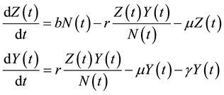
HIV transmission is not uniform between countries and among different stages of the disease within an infected individual [2] - [4] . As an infected person progresses from one stage of HIV infection to another, the level of transmitting the viruses to others changes. The transmission dynamics of the virus can be categorized into three stages of HIV progression of an infected individual [5] [6] . The first stage is the primary stage which follows soon after the initial infection. The second stage is the asymptomatic stage. In this stage, symptoms are few, and the patient’s blood contains a relatively small viral load and antibodies to the virus. The last stage is the symptomatic or AIDS stage. In this stage, an infected individual stays for a period of about 1 - 2 years until death, if no treatment is used.

Viral load varies greatly between these stages. During the period of primary infection, viral load is typically high. The viral load drops as one enters the asymptomatic period, followed by a symptomatic/AIDS stage during which the viral load is extremely high. A community-based study in which couples are prospectively followed for 30 months to evaluate the risk of transmission in relation to viral load and other characteristics shows that the risk of infection increases as an infected person’s viral load increases [2] . Another study also shows that the level of HIV infection is dependent on clinical status of the individual [7] . Most transmissions occur shortly after infection, after which infections become low until the immune system begins to be seriously affected.

The study of an epidemic, such as HIV, and its spread process in any community, is different to investigations in many other sciences. Data cannot be obtained through experiments in the population, but can only be obtained from surveys and results found in published or unpublished documents. These data are often not complete, may be inaccurate, and may vary with respect to methods used to collect them. Due to difficulties in obtaining HIV data, mathematical modelling and numerical simulation play an important role in analysing the behaviour of the epidemic, measuring its past, present, and future effect in a society.

Variations in the level of HIV transmission over time can have an impact on the estimates delivered from mathematical models. Existing models of transmission have either assumed a single group of infected individuals or have included stages of HIV progression to capture the transmission dynamics but have not studied how these two modelling approaches differ from each other. Lin et al. [8] studied a model that included stages of HIV progression in a general way. In a similar manner, McCluskey [9] [10] studied a similar model which was extended to include the effects of treatment. In all these models, none of them investigates the impact of including stages in the model and how the differences in the transmission among stages can have an impact on the results. In this work, the impact of including stages of HIV progression in models is investigated in order to understand how the model with and without stages affect the estimates produced.

2. Simple HIV Model

The HIV/AIDS model formulated here considers the total population, in a single homogeneous group divided into two subgroups: the susceptible population, , and infected individuals,. The demographics of the model are described by the rates of entry and exit of individuals from the population. The parameter b is the rate at which new individuals are recruited into the susceptible group, μ is the natural mortality rate (is the life expectancy of individuals), and is the rate at which infected individuals die from the disease.

The dynamics of the model are governed by the following system of differential equations:

(1)

where, r is the transmission rate and. From the above model, the total population change according to:

(2)

In this case, the total populations varies. This can be due to, or and. All parameters of the model are positive. The system is epidemiologically and mathematically well-posed in the sense that, if the initial data is a positive region in two dimension, the solutions remain defined for all in the same region.

Because varies over time, steady states are not expected in any parts of the population, but they may occur for the proportions. The model in Equation (1) is therefore converted into proportions. We define and to obtain:

(3)

which is positively invariant in the region:

Note that Equation (2) can be re-written as:

(4)

which integrates to:

(5)

indicating that when, the dynamics of the total population is strongly governed by the proportions of infected individuals in the population.

2.1. Existence of the Equilibria

This section derives stability conditions of the equilibrium points of the system in Equation (3).

Definition 2.1. Given a system of differential equations, an equilibrium point of this system is a point in the state space for which is a solution for all t.

We define a threshold factor:

(6)

from Equation (1) to represent the average number of secondary infections caused by one infective individual introduced into a completely susceptible population.

Theorem 2.2. For r > γ, the system in (3) always has a disease free equilibrium if and a unique endemic equilibrium point with and exist only if.

Proof. From the second equation of (3), with the right hand side equal to zero at large t, then equilibrium points must satisfy:

(7)

or

(8)

and

(9)

Substituting (7) and (8) in (9) or in the first equation of (3) with the right hand side equal to zero, gives or respectively. Equation (6) can be rewritten as. Substituting it in (8) gives. If, the only equilibrium in the region D is; if, the only equilibrium in D is. Therefore, the model has only two equilibrium points.

2.2. Stability Analysis

Local stability of the equilibrium points is performed by introducing of small perturbations, , at the equilibrium points as:

and substituting them in Equation (3). Because and are very small quantities, we discarding terms of higher order to obtain:

(10)

The coefficients of the perturbations give the Jacobian matrix:

. (11)

At the disease free equilibrium, the Jacobian matrix in (11) gives the following characteristic equation:

(12)

with eigenvalues and. If, both eigenvalues are real and negative and χ < 1. The disease free equilibrium become stable. If, then and the two eigenvalues have opposite signs. In this case, one solution approaches the equilibrium while the other moves away. The equilibrium point is therefore unstable.

Substituting the endemic equilibrium point, the Jacobian matrix gives the characteristic equation:

(13)

where,

(14)

(15)

(16)

and

If, it implies that. Therefore, the trace of the matrix, because

and the determinant, because

Thus, by the Routh-Hurwitz criterion, all of the eigenvalues have negative real parts and the endemic equilibrium point is stable. On the other hand, if, then and while, making one of the eigenvalue have a positive real part. Therefore, the endemic equilibrium point is unstable.

3. HIV Model with Stages

Here, the model in (0) is extended to include stages of HIV progression. The infected group is divided into two subgroups: those in the primary stage of HIV infection, and those in the asymptomatic stage,. The rate of progression from to is (assuming a constant rate) and is the time an infected individual spends in the primary stage (waiting times). Infected individuals in die at a rate. The dynamics are governed by the system:

. (17)

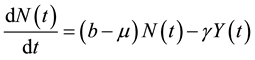
From the above model, the total population at time t is given by:

(18)

The parameters and determine transmission rates due the interaction between the susceptible individuals, and infected individuals in subgroups and, respectively. A study by Quinn et al [2] showed that transmission of the viruses from individuals in the primary stage to the individuals in the susceptible group is higher than those in the later stages. Therefore, in this model.

For stability analysis, the system in (17) is converted into proportions by letting, , and. Thus,

(19)

where

(20)

integrating to

(21)

The dynamic behaviour of the total population in this model is mainly governed by infected individuals who are in the asymptomatic stage of HIV infection,. This is because, it is only in this group individuals die from the disease.

Model (17) then becomes:

(22)

with

(23)

The above system have a positively invariant feasible region given by:

(24)

with all parameters positive.

The incidence of the disease is the proportion of new cases occurring in a population during a defined time interval. Using this model, incidence is given by:

(25)

where I is the incidence, and is the average time spent in the primary stage given by:

(26)

The prevalence of the disease is defined as the proportion of infected individuals in a population. From the model, prevalence is simply infected individuals in.

3.1. Existence of the Equilibria

Using the Next-generation technique [11] , the threshold quantity of the model is given by:

(27)

which is a linear combination of the threshold quantities of the infected individuals in the primary stage, and in the asymptomatic stage,. A factor is the probability that an infective individual will leave the primary stage of infection and enter the next stage (the asymptomatic stage).

Because of variable population size, system (22) is complex and calculation of the endemic equilibrium points is difficult. The dynamic behaviour of the population size (Equation (21)) is considered.

Definition 3.3. As, an equilibrium is reached and can be defined by, , and.

Theorem 3.4. The system in (22) has a unique endemic equilibrium point if the threshold quantity and a disease free equilibrium otherwise.

Proof. When the equilibrium is attained, the right hand side of system (22) goes to zero. Using the third equation in (22), we obtain:

(28)

Substituting (28) in the second equation of (22) while incorporating (23) gives:

(29)

where

(30)

Equation (29) gives always.

If, then (29) becomes:

(31)

But we know that, thus and

If then; if then. But also, since

, , and which makes the end points and for. Thus,

is a decreasing function. In this case,there is a unique root which accounts for the endemic equilibrium point when and a disease free equilibrium otherwise. ,

If the system approaches a disease free equilibrium, then (constant) asymptotically and the total population in Equation (21) change according to:

(32)

But in this case,. So, if, then decays asymptotically exponentially, remains constant if, and grows asymptotically exponentially if. Thus, since asymptotically, then from the third equation in (22), asymptotically and also by (23) and (24), asymptotically. Therefore, by 3.1, the disease free equilibrium.

If the system approaches the endemic equilibrium 3.2, then asymptotically with

. From (21), we have:

(33)

where and

(34)

decays asymptotically exponentially if, remains constant if, and grows asymptotically exponentially if c > 0. Since, then c ranges from when to when (i.e.).

From (34), we obtain. Substituting this in the third equation of (22), we get. By (23), which gives the endemic equilibrium.

3.2. Stability Analysis of the Equilibria

To analyze the stability of the equilibria, we establish a Jacobian matrix J and employ the Routh-Hurwitz technique to study the local stability of the equilibria. The Jacobian matrix of the system (22) is given by:

(35)

At the disease free equilibrium, (35) becomes:

(36)

From (36), and and are obtained from:

(37)

giving the characteristic equation:

(38)

The roots of (38) gives:

Clearly, always, and if, then. Under these conditions, the disease free equilibrium is stable. If, then either one or both and the disease free equilibrium is unstable.

Linearizing the model around the endemic equilibrium point, , the following characteristic equation is obtained:

(39)

where

with, , , , , , and. Since all model parameters are positive, then it is clear that, , , and. But also, if for, then, , , and. Under these conditions, , , and with are always positive. By the Routh-Hurwitz criteria, and by the Descartes rule of signs, the characteristic equation in (39) has roots with only negative real parts. Hence, the endemic equilibrium point is stable. If, then, , and. Therefore, the endemic equilibrium point is unstable.

4. Numerical Simulations

This section presents numerical simulation results of the models using parameter values described and presented in Section 4.1. We address the question whether it is necessary to incorporate stages of disease progression when modelling the spread of HIV/AIDS and seek to understand the effect of incorporating stages of HIV progression on the overall infection and spread of disease in the population as well as on estimation of future trend. In addition, we compare the two models by studying the effects of varying transmission rates on the models presented in this paper.

4.1. Model Parameterization

In sub-Saharan Africa, the average time lived by individuals is about 50 years. In this case, the natural mortality rate, is estimated to be 0.02 years⁻¹. In the same region, the average birth rate, b is estimated to be 0.03. Studies have also estimated the waiting times in the first stage of HIV is 2 to 10 weeks while individuals in the asymptomatic stage spend about 10 to 15 years [5] [6] .

On the other hand, the first empirical data in sub-Saharan Africa communities show substantial variations in transmission among stages of HIV infection after sero-conversion [2] [3] . These studies have showed that the rate of HIV transmission within the first two months is about 12 times higher than in the chronic stages. This indicates that transmission rate in the primary stage of HIV progression is higher than that of individuals in the asymptomatic stage.

The transmission rate, r as used in the simple model is estimated using the second equation in (3) at the steady state and given as:

(40)

where is the endemic equilibrium state of infections which takes any value in the interval. The minimum value that r takes when is and if then. Therefore,.

From the model with stages, is a function of. From second equation in (22) at equilibrium, and with gives:

(41)

where and c is given by Equation (34).

As the rate at which individuals become infected is increased, then and increases (Figure 1(a) and Figure 1(b)). This indicates that a careful choice of parameters r, and is required in models of HIV transmission. If the rates of infection are at their minimum values, the models show the disease to clear from the population (i.e.,) and the quantity become equal to one. According to the models, a disease persists in the population if the transmission rates are above their minimum values.

4.2. The Effect of Stages in HIV Predictions

Figure 2 presents numerical results of the models with and without stages. Because is as large as y since individuals in progress to within a very short period of time, we simulated the case where to compare the results of the two models. The results show a clear difference in the prevalence (and), and mortality (Figure 2(b) and Figure 2(c)). It is also observed that, prevalence is high for the model with stages and low for the model with a single group of infected individuals. increases just after the disease starts to exist. It is also observed that the effective threshold values () for the two models are different. For the model with stages, and for the model without stages,. The difference in is contributed by transmission of individuals in the primary stage (Figure 2(a)) as individuals in this stage have a high amount of viruses in the bloodstream, making transmission to others easier [2] [3] [5] [6] .

Because prevalence is high in infected individuals, mortality becomes high (Figure 2(c)). The difference in the mortality curves for the two models is similar to that found in the prevalence curves. The reason for this is that disease related mortality increase is proportional to the prevalence level in the population.

4.3. Effect of Transmission Rates

Figure 3 presents results of infected groups in the two models at different transmission rates. In general, the proportion of individuals in the infected groups increase with increasing the transmission rates. In the simple model, when r is increased from 0.167 to 0.5, increases from 1.28 to 3.85, and in the staged model, when is increased from 2.0 to 6.0, and from 0.167 to 0.5, increases from 1.61 to 4.82. Indicating that the transmission rates affect the results, especially when stages of disease progression are considered.

5. Summary and Conclusion

In this paper, a simple model for HIV transmission has been formulated and extended to incorporate stages of HIV progression. Stability analysis of the models and numerical simulation examples has been performed to understand the impact of stages in estimates. The effect of varying the transmission rates r, , and the disease related death rate () has been studied. The results show that the transmission rate is the driving force in the spread of the disease while the disease death rate has a generally little impact. Because of the sensitive effect of the transmission rates, incorporating stages in the model has a profound impact in the model results.

Our results indicate that when and are varied, a switch between the curves in occurs at large t. This is an interesting result which needs careful attention when dealing with disease incidence and transmission rate. One can easily draw different conclusions on the relation between the transmission rate and the persistence of new infections. This study has also shown that individuals in the primary stage play a major role in transmitting the disease. If this group can somehow be identified and convinced to refrain from risky behaviours, at least while they are highly infectious, the impact of the epidemic can be reduced.

The models produce different results. The model without stages produce estimates that are lower than the HIV estimates produced when stages are included. The nature of curves for y and is also different. In the model without stages, the curve for the proportion of infected people grows slowly than in the model with stages.

Although the models formulated are simple based on assumptions, and without fitting them to data, results show the importance of incorporating stages in models of HIV/AIDS. The results can not only be used to study how important stages of HIV infection are in the spread of HIV, but also they are helpful in evaluating the efficiency of HIV/AIDS models used in estimating and projecting the burden of HIV disease.

Acknowledgements

This work was developed from my MSc dissertation submitted to the University of Stellenbosch, South Africa with financial support from the African Institute for Mathematical sciences. The author acknowledges Fritz Hahne for valuable inputs.

Cite this paper

Angelina MageniLutambi, (2015) Modelling the Impact of Stages of HIV Progression on Estimates. Advances in Infectious Diseases,05,101-113. doi: 10.4236/aid.2015.53012

References

- 1. UNAID (2013) Global Report: UNAIDS Report on Global AIDS Epidemic 2013.
- 2. Quinn, T., Wawer, M., Sewankambo, N., Serwadda, D., Mangen, L.C.F., Meehan, M., Lutalo, T. and Gray, R. (2000) Viral Load and Heterosexual Transmission of Human Immunodeficiency Virus Type 1. The New England Journal of Medicine, 342, 921-929. http://dx.doi.org/10.1056/NEJM200003303421303
- 3. Wawer, M., Gray, R., Sewankambo, N., Serwadda, D., Li, X., Laeyendecker, O., Kiwanuka, N., Kigozi, G., Kiddugavu, M., Lutalo, T., Nalugoda, F., Mangen, F., Meehan, M. and Quinn, T. (2005) Rates of HIV-1 Transmission per Coital Act, by Stage of HIV-1 Infection, in Rakai, Uganda. Journal of Infectious Disease, 191, 1391-1393. http://dx.doi.org/10.1086/429411
- 4. Rapatski, B., Suppe, F. and Yorke, J. (2005) HIV Epidemics Driven by Late Disease Stage Transmission. Journal of Acquired Immune Deficiency Syndromes, 38, 241-253.
- 5. Perelson, A. and Nelson, P. (1999) Mathematical Analysis of HIV-1 Dynamics in Vivo. Society for Industrial and Applied Mathematics, 41, 3-44. http://dx.doi.org/10.1137/s0036144598335107
- 6. Witten, G. and Perelson, A. (2004) Modelling the Cellular-Level Interaction between the Immune System and HIV. South African Journal of Science, 100, 447-451.
http://reference.sabinet.co.za/document/EJC96305 - 7. Hyman, J., Li, J. and Stanley, A. (1994) Threshold Conditions for the Spread of HIV Infection in Age-Structured Populations of Homosexual Men. Theoretical Biology, 166, 9-31.
http://dx.doi.org/10.1006/jtbi.1994.1002 - 8. Lin, X., Hethcote, H. and Van Den Driessche, P. (1993) An Epidemiological Model for HIV/AIDS with Proportional Recruitment. Mathematical Biosciences, 118, 181-195.
http://dx.doi.org/10.1016/0025-5564(93)90051-B - 9. McCluskey, C. (2003) A Model of HIV/AIDS with Staged Progression and Amelioration. Mathematical Biosciences, 181, 1-16. http://dx.doi.org/10.1016/S0025-5564(02)00149-9
- 10. Guo, H. and Li, M.Y. (2011) Global Dynamics of a Staged-Progression Model for HIV/AIDS with Amelioration. Nonlinear Analysis: Real World Applications, 12, 2529-2540.
http://dx.doi.org/10.1016/j.nonrwa.2011.02.021 - 11. Van den Driessche, P. and Watmough, J. (2002) Reproduction Numbers and Sub-Threshold Endemic Equilibria for Compartmental Models of Disease Transmission. Mathematical Biosciences, 180, 29-48.
http://dx.doi.org/10.1016/S0025-5564(02)00108-6