Open Journal of Soil Science
Vol. 3 No. 2 (2013) , Article ID: 32580 , 10 pages DOI:10.4236/ojss.2013.32009
Evaluation of Soil Organic Carbon and Soil Moisture Content from Agricultural Fields in Mississippi
![]()
Department of Agricultural and Biological Engineering, Mississippi State University, Starkville, USA.
Email: *pparajuli@abe.msstate.edu
Copyright © 2013 Prem B. Parajuli, Sarah Duffy. This is an open access article distributed under the Creative Commons Attribution License, which permits unrestricted use, distribution, and reproduction in any medium, provided the original work is properly cited.
Received February 14th, 2013; revised March 15th, 2013; accepted March 24th, 2013
Keywords: Soil Organic Carbon; Soil Moisture Content; Cropland; Land Uses
ABSTRACT
Independent observation of the effects of agricultural management practices on soil organic carbon (SOC) with soil moisture content (SMC) is essential to quantify their potential relationships for sustainable ecosystems. Soil water retention studies and soil carbon stocks have been mapped in some areas worldwide. However, few studies have been conducted in the southeastern US, particularly in Mississippi. The objectives of this research study were to collect soil samples from fields chosen to be representative of the watersheds they are contained within, analyze the soil samples for carbon content and soil moisture content, and evaluate the relationship between SOC and different parameters (land use, vertical distribution, temporal distribution, and soil moisture content). Field sites were chosen based on their compositional similarity shared with the watershed as a whole in the Town Creek watershed (TCW) and Upper Pearl River watershed (UPRW) in Mississippi. Monthly soil samples from different depths (6 inch, 12 inch, and 24 inch) were collected from crop, pasture, and forest field areas. Soil samples were analyzed using bench analysis, elemental analysis, and statistical analysis. This study was able to demonstrate the SOC distribution in the soil layers across all three land uses studied. It was also shown that there does seem to be an interactive effect of parameters such as land use type, vertical distribution, and time on carbon accretion within the soil. Results of this study also determined that the near surface (6-in) layer was found to contain significantly more carbon than either the 12 inch or 24 inch layers (p < 0.01) across all field types. There was found to be a high degree of variability within the soil moisture data and correlation between SOC and SMC. It was found that carbon amount is not influenced by SMC but SMC could be influenced by SOC.
1. Introduction
In a modern world, teeming with an indifferent and expanding population, it has become imperative to study how human existence impacts the physical world in hopes of understanding how we might mitigate the strain on our planet. Carbon dioxide (CO2) is only one of the many critical variables under scrutiny given its exponential increase in the atmosphere over the last two centuries [1]. Rising CO2 concentrations are worrisome because of the serious threat it poses to global climate and ocean pH. However, it is anthropogenic activities that have easily overwhelmed the delicate balance that exists to keep the atmospheric CO2 concentration at innocuous levels.
One way to control and reduce greenhouse gas emission is through terrestrial carbon sequestration [2]. A plant removes CO2 from the atmosphere through photosynthesis whereby the CO2 is then broken down into carbon and oxygen. Oxygen is released into the atmosphere as waste while carbon is used for food and incorporated into the plant. As plants die or are harvested, the carbon-based leaves, stems, and roots decay in the soil, and the carbon becomes soil organic carbon (SOC). The SOC constitutes more than twice as much stored carbon as that of the earth’s vegetation and the atmosphere combined [3-5]. The SOC is estimated to be approximately 1500 Gigatonnes (Gt) globally [3,4,6]. SOC is strongly affected by human activity and its declining presence can be attributed to land conversion, soil disturbance, and increases in agricultural activity [6]. According to the US Environmental Protection Agency carbon sequestration rates vary by vegetative species, soil type, climate, topography and management practices [5]. A study estimated that anthropogenic pressures have caused the loss of anywhere between 42 and 78 Gt of soil’s original carbon content [7]. As startling as this assessment is, it also represents hope. The introduction of more judicious land management practices could have the capacity to increase SOC storage by an additional 0.4 - 1.2 Gt C⁄yr [6, 8]. This additional storage capacity in SOC represents the clear possibility that soils globally could considerably offset greenhouse gas emissions, namely CO2 [6,9,10]. However, “the present ability to forecast and improve the effects of climate and land cover change depends on SOC distributions, its control, source of inputs and outputs” [11].
An input of particular interest thought to have an interaction on SOC potential is soil moisture content (SMC). The SMC is an important parameter on its own, affecting runoff, land surface energy dynamics, and root zone productivity, and biomass yield [12,13]. Improved understanding and prediction of soil moisture can have far-reaching implications for irrigation planning, agricultural management, flooding and drought prediction, water quality assessment, and climate change [13]. A study compared several other studies done on the effects of SOC on SMC and found the results to be contradictory [14]. Soil carbon stocks and soil water retention studies have been mapped in some areas worldwide. However, few studies have been conducted in the southeastern US, particularly Mississippi. There have been some independent plot level studies done to observe the effects of agricultural management practices on carbon sequestration, but other variables interacting with the amount of SOC (such as SMC) have not been studied. The aims of this study were to: 1) examine the carbon content and soil moisture content of representative soil samples collected from two watersheds in central Mississippi; and 2) evaluate the relationship between SOC and different parameters (land use, vertical distribution, temporal distribution, and soil moisture content). By choosing sites that are compositionally similar to the watershed as a whole, the sites act as micro-watersheds that offer the potential to be scaled up and modeled. Long-term soil and land management datasets, in addition to model estimates, could provide valuable resource information to land managers and policy makers.
2. Materials and Methods
2.1. Study Area
The focus areas of this study were in two agricultural watersheds: Town Creek watershed (TCW) and Upper Pearl River watershed (UPRW). Watershed areas of the TCW is about 177,500 ha (438,612 ac) and UPRW is about 360,863 ha (891,711 ac). The TCW is located within Lee, Union, and Pontotoc counties with little areas in Chickasaw, Monroe and Itawamba counties (Figure 1). According to climate data the mean annual precipitation for the TCW is estimated as 154 cm, mean monthly minimum temperature of −19˚C and a maximum temperature of 42˚C [15]. Surface elevation of the TCW ranges from 48 m to 241 m with about 999 farms [16]. The Town Creek starts near Sherman and drains south of Nettleton [17].
The UPRW covers about ten counties (Attala, Choctaw, Kemper, Leake, Madison, Neshoba, Newton, Noxubee, Scott, and Winston; Figure 2). According to climate data the mean annual precipitation for the UPRW is estimated as 142 cm, mean monthly minimum temperature of −18˚C and a maximum temperature of 41˚C in August with a mean annual temperature of 17.7˚C

Figure 1. Location map of the Town Creek watershed in NE Mississippi.
[15]. Surface elevation of the UPRW ranges from 50 m to 221 m. The UPRW is classified as forested watershed with good livestock population [18]. The Pearl River starts near Nanih Waiya Indian mounds in Winston County and drains in the Ross Barnett Reservoir [19].
2.2. Site Selection
Study fields were chosen based on characteristics which are typical of each study watershed. Details of the locations and characteristics for each sampling point are summarized in Table 1 and are pictured in Figures 3 and 4. TCW has six sampling points all in crop land use while the UPRW has six points split between forestland and pastureland. All study areas were located on privately owned property and sampling was conducted with the permission of the landowners. In the TCW two crop fields with historical corn-soybean plant rotations were chosen. Field 1 is 22 ha (54 ac) and has been harvested the last 30 years with a corn-soybean rotation. Field 2 is approximately 121 ha (300 ac) that has been planted with corn, soybeans and cotton for the last 20 years. Both properties are directly adjacent to Town Creek within the watershed.
In the UPRW a representative forest area (Field 3) and pastureland (Field 4) were chosen. Field 3 is a 2 ha (5 ac) pine plantation that was planted for the first time five years ago with 0.2 ha (0.5 ac) harvested in summer 2011. Previous to the pines, the field served as an open pasture. Field 4 is approximately 6 ha (15 ac) and currently has 10 head of cattle and one donkey that use the area as their primary grazing location.
Three points were chosen arbitrarily at each field location and identified as Point 1 through Point 12. In Fields 1, 2 and 3, the sampling area considered for the location of the points was limited to areas with close proximity to the field entrance due to the potential issues of accessing the points during peak crop growth.
2.3. Soil Physical and Hydraulic Properties
The physical and hydraulic properties of each field are shown in Table 2. Fields 1 and 2 in the TCW consist of Catalpa soil (MUID MS117). The Catalpa series, identified in Oktibbeha County, Mississippi in 1907, consists of deep, somewhat poorly drained to moderately welldrained silty clay loam and silty clay soils [21]. Slopes range from 0 to 3 percent, and the soil ranges from slightly acid to moderately alkaline. Most areas that consist of this soil series have been cleared and are used for growing pasture, hay, and row crops such as cotton, corn, and soybeans [21]. Determination of this soil type was based on data from the US General Soil Map (STATSGO2) [22].
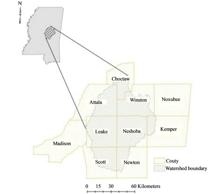
Figure 2. Location map of the Upper Pearl River watershed in central Mississippi.

Table 1. Locations of sampling points.
 Fields 1
 Fields 2
Figure 3. Aerial imagery of Fields 1 and 2 located in TCW. Fields are outlined in orange and point locations 1 - 6 are noted [20].

Figure 4. Aerial imagery of Fields 3 and 4 located in the UPRW. Fields are outlined in orange and point locations 7 - 12 are identified [20].
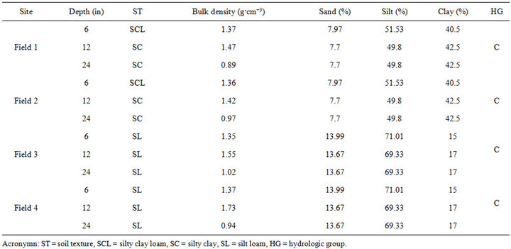
Table 2. Physical and hydraulic properties of the soils.
Fields 3 and 4 are composed of Ariel soil (MUID MS059 and MS067, respectively). The Ariel series consists of deep, well drained, nearly level silty loam soils on flood plains and low stream terraces with slopes ranging from 0 to 2 percent [23]. Most areas of Ariel soil are used for pasture and a small percentage is woodland [23]. Soil type determination was based on data from the US General Soil Map (STATSGO2) [22].
2.4. Soil Sampling
Earlier studies have shown that land use related change in soil properties is most strongly affected in the top surface layers [6]. As such, it was determined that soil cores would be taken at depths of 0 - 6 in, 6 - 12 in, and 12 - 24 in. Soil cores at the prescribed depths were collected once monthly at all twelve points. Samples were extracted using a thin-walled stainless steel T-handle soil probe (Forestry Suppliers Inc., item number 77654) of 11/16-in diameter with careful efforts made to minimize contamination between layers during extraction. Soil samples were collected in zipping plastic bags and were stored in cool (<21˚C) dark conditions until they could be processed. During the course of the study there were three months when data was not collected at Fields 1 and 2 (January 2011, April 2011, and August 2011) or at Fields 3 and 4 (November 2010, January 2011, and August 2011).
2.5. Soil Analysis
Bench Analysis. The bench analyses were performed in the Agricultural and Biological Engineering Water Quality Laboratory at Mississippi State University. To prepare the samples for dehydrating, the samples were transferred from plastic bags to standard paper bags. The samples were weighed (“wet weight”) and then placed in a thermostatically controlled Grieve welded steel laboratory oven (Model LO-201C). Samples were dried at a temperature of 60˚C ± 5˚C for 24 hours. The samples were then weighed again (“dry weight”) whereby their soil moisture percentage could be calculated (Equation 1).
 (1)
(1)
Bulk density was determined on individual samples by dividing the oven-dry weight of the sample by the volume of the soil probe at the respective depth (see Equation (2)). The average bulk density based on depth was then taken for each field.
 (2)
(2)
Soil densities vary over a wide range, and typically between 0.1 g·cm−3 for light peats and 1.8 g·cm−3 for very dense, compacted mineral soils with little pore space [24].
Elemental Analysis. Dry combustion using an elemental analyzer is the most accurate standard laboratory test for soil carbon, and is based on a solid-to-gas transformation by flash combustion of the sample material and measurement of concentrations via gas chromatography [24].
In this study samples from the same field were composited based on depth in order to achieve an average across the field at each respective depth. Once aggregated the samples were finely ground using a Dynacrush Soil Crusher (Custom Laboratory Equipment Inc., Orange City, FL). Pulverization was done until a majority of the sample could pass through a 60-mesh sieve. Sieving helped to ensure particles were 250 µm or less and also aided in the complete removal of any stray litter that may have been erroneously captured in the sample. A portion of the pulverized sample was then transferred to a 4 milliliter glass vial and dried at 105˚C for one hour to remove any latent moisture acquired during pulverization. A subsample of approximately 30 milligrams was then measured out and sealed into an ultra-pure 5 × 9 mm tin capsule. The tin capsules were then loaded into a rotating autosample carousel and analyzed for carbon content using a Costech 4010 CHNS Dry Combustion Analyzer [25].
The Costech 4010 CHNS Dry Combustion Analyzer works by delivering one sample at a time into a 1050˚C chromium oxide combustion reactor, pushed along by a helium carrier stream mixed with excess oxygen. Under these conditions, the tin capsule undergoes a flash combustion which raises the sample temperature to as much as 1800˚C, forming water, CO2, and nitrogen gas (N2). Carbon content from the soil sample is changed to CO2 during flash combustion. Water content from the soil sample is removed by a gas trap having magnesium perchlorate. Generally, clean gases from the sample are passed through a gas chromatograph column to separate the N2 and CO2. More chemical processes and analysis are described in the combustion analyzer document [25].
Calibration for the Costech 4010 CHNS system was performed using a standard procedure [25] using a LECO standard. In this particular study standards were measured in five increments (0.10, 0.20, 0.30, 0.45 and 0.60 micrograms) to generate the calibration curve; total C and total N content values were calculated using the standard chemical formulae and are entered before testing begins. In every ten samples an empty tin capsule blanks were used. Any detectable nitrogen or carbons in these blanks were subtracted from the sample to have a zero baseline. The correction for C traces were created from the tin capsules by blanks and for the small amount of N2 gas introduced as an impurity in the oxygen pulse [25].
2.6. Statistical Analysis
Arithmetic means and standard deviations were calculated on the SOC data and SMC data collected from each field. Significance of the fixed effects of land use, depth of sample, sampling date, and SMC, and their interactions were analyzed using the generalized linear mixed model (GLMM) procedure (GLIMMIX) embedded in SAS software [26]. The GLMM was chosen due to its ability to model “data with correlations or nonconstant variability and where the response is not necessarily normally distributed” [26].
3. Results and Discussion
3.1. Carbon Analysis
Mean values and associated standard deviations of the SOC (percentage of carbon in the sample) are presented in Tables 3 and 4. Samples collected between September 2010 and February 2012 from four study sites at depths of 6 inch, 12 inch, and 24 inch were analyzed for percent carbon content using an elemental analyzer. Results were found to be consistent with the earlier studies in that the near surface (6-in) layer was found to contain significantly more carbon than either the 12- or 24-in layers (p < 0.01) across all field types [6,11]. Also as expected, the deeper layers show less variation with time. Furthermore, it was found that carbon amount was relatively consistent throughout the duration of the study period.
3.2. Soil Moisture
Mean values and associated standard deviations of the SMC (percentage of water in the sample) are presented in Tables 5 and 6. Soil moisture measurements were made on soil cores taken from the four field locations. There was found to be a high degree of variability within the soil moisture data. Across the entire dataset, there was
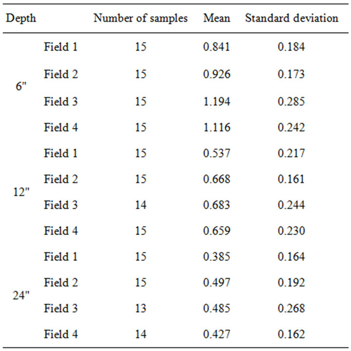
Table 3. Means and standard deviations of percent carbon based on field.

Table 4. Overall means and standard deviations of percent carbon based on depth.
found to be a variance of 58.35 which is very high. This could be attributed to the inherent variability in collection dates after rain events or local variability of rain events (rain occurring at one site and not another). Because SMC was calculated as a percentage, sample size was not an attributing factor to the variability. Mean values and associated standard deviations of the SMC (percentage of water in the sample) are presented in Tables 5 and 6.
3.3. Interaction of Parameters
Secondary to the carbon content and SMC analyses which were the main justification for this portion of the study, fixed factors associated with each sampling location were analyzed to determine the degree to which they influenced carbon amount. Fixed factors included land use, depth of sample, time, and SMC. Although it is known that soil carbon content is the result of a myriad of factors, including soil physical and hydraulic properties, it was thought that there might be statistical evidence of interaction when carbon content was compared to the factors listed above. Already noted was a significant correlation of SOC and depth.
The statistical analysis procedures used for this portion of the study were the GLIMMIX and correlation procedures using SAS software. A univariate analysis was also performed on the carbon values to confirm that the distribution of the data was within acceptable range. The variable of interest is skewness and ideally it should be between −1 and 1. The carbon values for this dataset (n = 176) had a skew of 0.60 so no transformation of the data was necessary. Initially, a full model was run including all of the potential factors. The purpose of this was to identify the complexities of the responses (Table 7).
Several factors of the linear mixed model namely, field type (“Field”), sample depth (“Depth”), field by depth (“Field*depth”), time (“Mon”), sampling date by depth (“Mon*depth), and sampling date by sampling date (“Mon*mon”), were found to be significant (p < 0.05).
Given the above, the next step was to simplify the analysis by isolating one variable and analyzing it at each level while everything else remained unchanged. A general statement about the four fields cannot be made because each field has its own characteristics. Therefore, the next model examined each depth (6, 12, and 24) at

Table 5. Means and standard deviations of SMC (percent) based on field.

Table 6. Overall means and standard deviations of SMC (percent) based on depth.

Table 7. Full GLIMMIX model results showing factors and the complexity of their response.
every field. At 6 in there were found to be linear effects as a result of field and time. LS Means (α = 0.05) groupings of Fields 3 and 4 in A and Fields 2 and 1 in B. At 12 inches, responses were more complex; there was a linear effect of time and quadratic response over time. For this analysis, LS means (α = 0.05) groupings were not significantly different for any of the fields (all A grouping). At 24 inches across all fields a linear time effect was the only significant factor. Again, all LS means (α = 0.05) groupings were not significantly different for any of the fields (all A grouping).
Then the reverse of the above was done first separating field type and then depth within every field. The effect of depth and time were highly significant at all four fields. Fields 2 and 4 also showed a quadratic response over time. LS means (α = 0.05) groupings show significance of depth at each level: 6 inches = A, 12 inches = B, and 24 inches = C for Fields 1, 2 and 3. All four fields were found to have a difference of carbon concentration with depth but the means are different and concentration varies over time (three were linear and one was not).
Field type does have an effect at 6 inches but not at 12 inches or 24 inches as concluded by the depth analysis. The second analysis determined that two of the fields are the same but the other two are unique. Finding an effect of land use in the surface layer was consistent with what was reported by earlier study [6]. The results of both of these analyses meant further analysis to examine each depth in order to develop a mathematical model to predict carbon content. The coefficient of determination (R2) was used to evaluate the efficacy of the equation to the observed data.
For the regression analysis the fields were recorded. Since the previous analysis determined there was not a statistical difference between Fields 1 and 2 (crop) or Fields 3 and 4 (non-crop) at the 6 inch depth, recoding reduced the data to two levels. At depths of 12 inches and 24 inches all fields were considered as one since there was no effect of field type on carbon content at those depths. The regression analysis consisted of fitting the best models to determine the regression equations. Regression equations derived from the models are as follows and are represented graphically in Figure 5:
Crop fields at 6 in: carbon concentration = 1.125 – 0.0281*time.
Non-crop fields at 6 in: carbon concentration = 1.39 – 0.0281*time.
All fields at 12 in: carbon concentration = 0.9567 – 0.07795*time + 0.00368*time2.
All fields at 24 in: carbon concentration = 0.5717 – 0.01442*time.
The R2 values for each of the equations were 0.52, 0.22, and 0.12 respectively. All fields showed a carbon response over time. The linear response over time at the 24 in depth was not highly significant (significant at 0.05 level not 0.01). Therefore, this model may be statistically significant but biologically questionable. It is noteworthy to mention that R2 is a function of how steep the line is (less slope means lower R2). It is evident that Fields 3 and 4 contain higher carbon content than the combined crop fields and all fields at the 6 inch depth contain more carbon compared to all fields at 12 inch or 24 inch depths. These results are in accordance with other studies [11]. The fact that the carbon concentration is decreasing with time is unexpected. It is likely the decrease of carbon over time is a result of user error when analyzing for
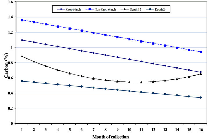
Figure 5. Regression plots using GLM model for all three depths.

Figure 6. Correlation plot of carbon content (%) and SMC (%) across all fields at all depths (n = 176). No linear correlation exists.
carbon content and not a change that is occurring in situ.
A correlation procedure was performed on the carbon data and SMC data to determine if there was a relationship between the two variables. The reported correlation measures for the entire dataset (all fields and all depths) show a slight (but not significant according to the p-value) positive correlation between SMC and carbon amount (0.10). The correlation at Fields 3 and 4 at the 6 inch depth were 0.25 and 0.41 respectively. Correlation for Fields 1 and 2 (combined) was close to 0 (0.0041) and was not significant. Figure 6 is a plot of the entire dataset (n = 176). This graph illustrates minimal correlation between the two variables of interest (SMC on the x-axis and carbon content on the y-axis). When graphed this way, it is apparent that there is no visual linear relationship between the two variables and the low R2 confirms lack of correlation.
4. Conclusions
This study was able to demonstrate that the majority of SOC is contained within the near surface layer of soil across all three land uses studied. It was also shown that there does seem to be an interactive effect of parameters such as land use type, vertical distribution, and time on carbon accretion within the soil. There was found to be significantly more carbon in the forestland (Field 3) and pastureland (Field 4) at 6 inches than combined croplands possibly due to fewer disturbances in the soil column. A decrease in carbon amount was seen over time using regression models but this was likely a result of user error. There was no statistically significant correlation between carbon content and SMC although correlation (or lack thereof) does not imply causation.
These results are reasonable since the amount of SOC is dependent on the source input of carbon and well as management pressures. Since there were only 13 to 15 months of samples for each field, results may change as sample size increases. It was also found that carbon amount is not influenced by SMC but SMC could be influenced by SOC.
5. Acknowledgements
This material is based upon work performed through the Sustainable Energy Research Center at Mississippi State University and is supported by the Department of Energy under Award Number DE-FG3606GO86025; Micro CHP and Bio-fuel Center. We acknowledge the contributions of Jeffery Hatten in the Dept. of Forestry at Mississippi State University and landowners of the research fields in the watershed for this research.
REFERENCES
- D. Reay and M. Pidwirny, “Carbon Dioxide,” In: C. J. Cleveland, Ed., Encyclopedia of Earth, 2011. http://www.eoearth.org/article/Carbon_dioxide
- V. Yadav, G. P. Malanson, E. Bekele and C. Lant, “Modeling Watershed-Scale Sequestration of Soil Organic Carbon for Carbon Credit Programs,”. Applied Geography, Vol. 29, No. 4, 2009, pp. 488-500. doi:10.1016/j.apgeog.2009.04.001
- N. H. Batjes, “Total Carbon and Nitrogen in the Soils of the World,” European Journal of Soil Science, Vol. 47, No. 2, 1996, pp. 151-163. doi:10.1111/j.1365-2389.1996.tb01386.x
- R. A. Houghton, “The Contemporary Carbon Cycle,” In: W. H Schlesinger, Ed., Biogeochemistry, Elsevier Science, 2005, pp. 473-513.
- US Environmental Protection Agency (USEPA), “Carbon Sequestration in Agriculture and Forestry,” 2011. http://www.epa.gov/sequestration/tools_resources.html
- B. R. Wilson, T. B. Koen, P. Barnes, S. Ghosh and D. King, “Soil Carbon and Related Soil Properties along a Soil Type and Landuse Intensity Gradient, New South Wales, Australia,” Soil Use and Management, Vol. 27, No. 4, 2011. pp. 437-447. doi:10.1111/j.1475-2743.2011.00357.x
- R. Lal and R. F. Follett, “Soil Carbon Sequestration and the Greenhouse Effect,” 2nd Edition, Soil Science Society of America, Madison, 2009.
- R. Lal, “Soil Carbon Sequestration Impacts on Global Climate Change and Food Security,” Science, Vol. 304, No. 5677, 2004. pp. 1623-1627. doi:10.1126/science.1097396
- S. M. Ogle, F. J. Breidt, M. D. Eve and K. Paustian, “Uncertainty in Estimating Land Use and Management Impacts on Soil Organic Carbon Storage for US Agricultural Lands between 1982 and 1997,” Global Change Biology, Vol. 9, No. 11, 2003. pp. 1521-1542. doi:10.1046/j.1365-2486.2003.00683.x
- K. Y. Chan, M. K. Conyers, G. D. Li, K. R. Helyar, G. Poile, A. Oates and I. M. Barchia, “Soil Carbon Dynamics under Different Cropping and Pasture Management in Temperate Australia: Results of Three Long-Term Experiments,” Soil Research, Vol. 49, No. 4, 2011. pp. 320-328. doi:10.1071/SR10185
- E. G. Jobbágy and R. B. Jackson, “The Vertical Distribution of Soil Organic Carbon and Its Relation to Climate and Vegetation,” Ecological Applications, Vol. 10, No. 2, 2000, pp. 423-436. doi:10.1890/1051-0761(2000)010[0423:TVDOSO]2.0.CO;2
- M. S. Moran, C. D. Peters-Lidard, J. M. Watts and S. McElroy, “Estimating Soil Moisture at the Watershed Scale with Satellite-Based Radar and Land Surface Models,” Canadian Journal of Remote Sensing, Vol. 30, No. 5, 2004, pp. 805-826. doi:10.5589/m04-043
- E. Han, “Soil Moisture Data assimilation at Multiple Scales and Estimation of Representative Field Scale Soil Moisture Characteristics,” Ph.D. Thesis, Purdue University, West Lafayette, 2011.
- W. J. Rawls, Y. A. Pachepsky, J. C. Ritchie, T. M. Sobecki and H. Bloodworth, “Effect of Soil Organic Carbon on Soil Water Retention,” Geoderma, Vol. 116, No. 1-2, 2003, pp. 61-76. doi:10.1016/S0016-7061(03)00094-6
- National Climatic Data Center (NCDC), “Locate Weather Observation Station Record,” 2011. http://www.ncdc.noaa.gov/oa/climate/stationlocator.html
- Natural Resources Conservation Service (NRCS), “Mississippi Conservation Security Program (CSP),” 2011. http://www.ms.nrcs.usda.gov/programs/MissCSP.html
- US Environmental Protection Agency (USEPA), “Waterbody Report for Town Creek,” 2006. http://oaspub.epa.gov/tmdl/attains_waterbody.control?p_list_id=MS013TE&p_cycle=2006&p_state=MS&p_report_type=T
- US Department of Agriculture, National Agricultural Statistics Service (USDA-NASS), “Mississippi County DataLivestock.United States Department of Agriculture (USDA),” 2011. http://www.nass.usda.gov/Statistics_by_State/Mississippi/Publications/County_Estimates/index.asp
- Pearl River Basin Development District (PRBDD), “Pearl River Basin Development District: Topography and History,” 2011. http://www.pearlriverbasin.com/topography_and_history.php
- Google Inc., “Google Earth (Version 6.2.2.6613) [Software],” 2012. http://www.google.com/earth/index.html
- M. C. Garber, “Soil Survey for Lee County Mississippi,” United States Department of Agriculture, Soil Conservation Service, US Government Printing Office, 1973, p. 8.
- US Department of Agriculture, Natural Resources Conservation Service (USDA-NRCS), “US General Soil Map (STATSGO2) for Mississippi,” 2006. http://soildatatmart.nrsc.usda
- F. T. Scott, “Soil Survey for Madison County, Mississippi,” United States Department of Agriculture, Natural Resource Conservation Service, US Government Printing Office, 1984, pp. 2-13.
- P. Donovan, “Measuring Soil Carbon Change: A Flexible, Practical, Local Method,” 2012. http://soilcarboncoalition.org/taxonomy/term/2
- Costech Instruments, “Elemental Combustion System CHNS-O,” 2006. www.costechanalytical.com
- SAS Institute Inc., “The GLIMMIX procedure,” 2006. http://support.sas.com/rnd/app/papers/glimmix.pdf
NOTES
*Corresponding author.