ABSTRACT

Consider a first-order autoregressive processes, where the innovations are nonnegative random variables with regular variation at both the right endpoint infinity and the unknown left endpoint θ. We propose estimates for the autocorrelation parameter f and the unknown location parameter θ by taking the ratio of two sample values chosen with respect to an extreme value criteria for f and by taking the minimum of over the observed series, where represents our estimate for f. The joint limit distribution of the proposed estimators is derived using point process techniques. A simulation study is provided to examine the small sample size behavior of these estimates.

1. Introduction

In many applications, the desire to model the phenomena under study by non-negative dependent processes has increased. An excellent presentation of the classical theory concerning these models can be found, for example, in Brockwell and Davis [1]. Recently, advancements in such models have shifted focus to some specialized features of the model, e.g. heavy tail innovations or nonnegativity of the model. In this paper we examine the behavior of traditional estimates under conditions leading to non-Gaussian limits. For example, the standard approach to parameter estimation within the AR(1) process is through the Yule-Walker estimator;

(1.1)

A slightly different approach presented in Mathew and McCormick [2] used linear programming to obtain estimates for and under certain optimization constraints. While there are many established methods to estimate the autocorrelation coefficient in an AR(1) model, there are just a few approaches on estimating the unknown location parameter in an AR(1) model. Onewas mentioned in McCormick and Mathew [2] where they considered

and provides the index of the maximal and minimal respectively for.

In this paper we examine estimation questions and asymptotic properties of alternative estimates for and respectively, relating to the model

where and is an i.i.d. sequence of nonnegative random variables whose innovation distribution F is assumed to be regularly varying at infinity with index and regularly varying at with index, where, denotes the unknown but positive left endpoint. As a result of not restricting the innovations to be bounded on a finite range, we can first estimate the autoregressive parameter through regular variation at infinity and then estimate the positive but unknown location parameter through regular variation at, the left endpoint.

While we have mentioned a few established estimation procedures, one notable exception was that of maximum likelihood. Although typically intractable and intricate in the time series setting, when the innovations in the AR(1) model are exponential, the maximum likelihood procedure had a major contribution on the estimation of positive heavy tailed time series. With these considerations in mind, Raftery [3] determined the limiting distribution of the maximum likelihood estimate for the autocorrelation coefficient. As a result, the estimator

(1.2)

was considered. The realization of this estimator was the stepping stone for the work done in this paper along with Davis and McCormick [4] which first considered this alternative estimator and used a point process approach to obtain the asymptotic distribution of the natural estimator. This was done in the context that the innovations distribution varies regularly at 0, the left endpoint, and satisfy some moment condition.

The work presented in this paper is an extension of the work done in Davis and McCormick [4] including the following contributions to dependent time series with heavy-tail innovations. The first contribution involves the development of estimates for the autocorrelation coefficient and unknown location parameter under regular variation at both endpoints, with a rate of convergence, where is slowly varying function. The second contribution involves using an extreme value method, e.g. point processes to establish the asymptotic distribution of the proposed estimators and weak convergence for the asymptotically independent joint distribution. An initial observation is that our estimation procedure is especially easy to implement for both and. That is, the autoregressive coefficient in the causal AR(1) process is estimated by taking the minimum of the ratio of two sample values while estimation for the unknown location parameter was achieved through minimizing over the observed series.

This naturally motivates a comparison between the estimation procedure presented in this paper and the standard linear programming estimates mentioned above, since within a nonnegative AR(1) model the linear programming estimate reduces to the estimate proposed, namely, , where denotes the AR(1) process. This comparison along with the comparison between Mathew and McCormick’s [2] optimization method and Bartlett and McCormick [5] extreme value method was performed through simulation and is presented in Section 3. The results found appear to demonstrate a favorable performance for our extreme value method over the 3 alternative estimators.

The main proofs in this paper rely heavily on point process methods from extreme value theory. The essential idea is to first establish the convergence of a sequence of point processes based on simple quantities and then apply the continuous mapping theorem to obtain convergence of the desired statistics. More background information on point processes, regular variation, and weak convergence can be found in Resnick [6]. Also, a nice survey on linear programming estimation procedures and nonnegative time series can be found in Anděl [7], Anděl [8], and Datta and McCormick [9], whereas more applications on modeling the phenomena with heavy tailed distributions and ensuing estimation issues can be found in Resnick [10].

The rest of the paper is organized as follows: asymptotic limit results for the autocorrelation parameter, unknown location parameter, and joint distribution of are presented in Section 2, while Section 3 is concerned with the small sample size behavior of these estimates through simulation.

2. Asymptotics

The following point process limit result is fundamental. Since the result makes no use of an ARMA structure, we present it for more general linear models subject to usual summability conditions on the coefficients. In that regard for this result, we assume that is the stationary linear process given by

with for some. Furthermore for this result we may relax our assumptions on the innovation distribution and we require that has a regularly varying tail distribution, i.e.,

for a slowly varying function and the innovation distribution is tail balanced

Define point processes

and let denote PRM on where

has Radon-Nikodym derivative with respect to Lebesgue measure

Let be an iid array with and independent of. Define

Our basic result is to show that equipped with the topology of vague convergence

which is close in statement and spirit to Theorem 2.4 in Davis and Resnick [11]. In view of the commonality of the two results, we present only the needed changes to the Davis and Resnick proof to accommodate the current setting. Aside from keeping track of the time when points occur, i.e. large jumps, the difference in the point processes considered here with those in Davis and Resnick [11] is the inclusion of marks, i.e. the second component of the point. This complication induces an additional weak dependence in the points which is addressed in Lemma 2.2 through a straight forward blocking argument. First, we establish weak convergence of marked point processes of a normalized vector of innovations. For a positive integer m define

and point process

Let denote the standard basis vectors for. Define an associated marked point process with the first component placed on an axis by

In the following Lemma, we show that and are asymptotically indistinguishable in the following sense. Let and. Consider the class of rectangles

Lemma 2.1. As tends to infinity

.

Proof. Following the proof presented in Proposition 2.1 of Davis and Resnick [11], suppose that is such that for some As noted in Davis and Resnick [11] for all, one has. Observe that

(2.1)

Similarly let and. Then

(2.2)

where according to and. Note that

(2.3)

Thus from (2.1)-(2.3) we obtain

(2.4)

Then the result follows as in Davis and Resnick [11], Proposition 2.1, completing the proof. □

Lemma 2.2. Let and be the point processes on the space defined by

where is an iid sequence with

and is independent of. Then in,

Proof. We employ a blocking argument to establish this result. Let be a sequence of integers such that as and. Let and. Define blocks

Then it is clear that for

Write

Then

(2.5)

Let be a disjoint union of rectangles

(2.6)

where with. Let denote the mean measure of which is PRM on. To complete the proof we first show that for all sets of the form given in (2.6) that

(2.7)

The above limit result follows from the easily verifiable relations:

(2.8)

(2.9)

(2.10)

(2.11)

and

(2.12)

Indeed, in view of (2.5) and (2.12), (2.7) is equivalent to showing

(2.13)

and the above relation holds by (2.8), (2.10), and (2.11), viz.

It is immediate that for a rectangle

we have

(2.14)

Therefore the result is seen to hold by (2.7) and (2.14) by application of Theorem 4.7 in Kallenberg [12]. □

Lemma 2.3. Let and be point processes on the space

Then in,

Proof. We begin by applying the argument used in Theorem 2.2 of Davis and Resnick [11] with the modification that the relevant composition of maps of point processes is given by

Each map being continuous, the composition is a continuous map from to with each space being equipped with the topology of vague convergence. Therefore by the continuous mapping theorem and Lemma 2.2 we obtain

(2.15)

Finally we complete the proof by Lemma 2.1 and (2.15) arguing as in Davis and Resnick [11].

We are now ready to present our fundamental result.

Theorem 2.1. Let and be the point processes on the space defined by

where is and is an iid array with and independent of.

Then in

Remark. Apart from considering a time coordinate and restricting the process to an AR(1) process, the above Theorem 2.1 and Theorem 3.1 in Mathew and McCormick [2] consider essentially the same point process limit result. However, their result gave a wrong limit point process. This error is corrected in the current paper.

Proof. Observe that the map

induces a continuous map on point processes given by

Thus we obtain from Lemma 2.3 that

(2.16)

The result now follows from (2.16) by the same argument in Davis and Resnick [11] to finish their Theorem 2.4.

Returning to the AR(1) model under discussion in this paper and the estimate given in (1.2), we obtain the following asymptotic limit result.

Theorem 2.2. Let be the stationary solution to the AR(1) recursion and

. Under the assumptions that

and the innovation distribution F has regularly varying right tail with index and finite positive left endpoint,

where and.

Proof. For define a subset

Then note that for the point processes

, we have

Applying Theorem 2.1 in the case of an AR(1) process so that, we have

Note that as a subset of, the set is a bounded continuity set with respect to the limit point process so that

where is an i.i.d. sequence independent of. Let

(2.17)

Then by Proposition 5.6 in Resnick [10], we have that if denotes the distribution of, then is a Poisson random measure on E with mean measure, where. Using (2.17) we can write

Since, the result follows.

Corollary 2.1. Under conditions given in Theorem 2.2,

Proof. Since we have

. But this implies since

and is non-increasing.

Let us now define our estimate of:

where we define the index set

where

is a fixed value.

Lemma 2.4. Under the assumptions that F is regularly varying with index at its positive left endpoint and is regularly varying with index at infinity, its right endpoint, and, then

where. Furthermore, for any

Proof. Since, we have.

Therefore since is a tight sequence by Theorem 2.2 and since with

, we have

The first statement now follows since

For the second statement observe

(2.18)

The result for the second statement now follows from (2.18) and the first part of the lemma. Finally, the identification of the limit distribution is well known. □

A useful observation follows from this lemma which we state as a corollary.

Corollary 2.2. Under the assumptions of Lemma 2.4 for any

Proof. By Lemma 2.4 we have

The result then follows from

□

Corollary 2.2 allows a simplification in determining the joint asymptotic behavior of by allowing us to replace with. The next lemma will provide another useful simplification—this time on.

For a positive integer define

Lemma 2.5. Let and be defined as

Then for any

Proof. We first note for any positive that

In order to calculate we partition

. That is, we write

where, so that

Define point processes

where and have the distributional properties given in Theorem 2.2. Applying Theorem 2.2 with for and equal to 0 otherwise, we obtain

Then letting for

we have

Setting

we have

where

Since is Poisson random measure with mean measure where and

we obtain

Next since

we have for large n that

Therefore, since,

Next, note that from the limit law for the maximum obtained above, by replacing with and by taking reciprocals, we derive the limit law for minimum,

(2.19)

where has the distribution of. Thus, for any integer,

Thus for any, we have for large enough that

completing the proof. □

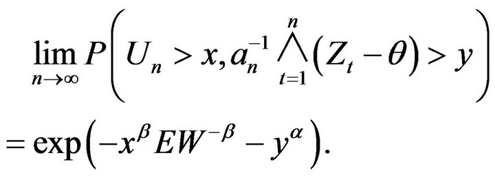
With Lemma 2.5 in hand we can now focus our attention to the limiting joint distribution of.

This will be accomplished by a blocking argument. To that end for a fixed positive integer, let and define blocks for by

where is a positive integer greater than. Furthermore, let

Now we define the events

and

where. We begin by showing that the events are negligible.

Lemma 2.6. For any

Proof. Observe that

(2.20)

and

(2.21)

Thus for some constant and any,

establishing the lemma.

Define events and by

The following result provides the asymptotic behavior of the probability of these events.

Lemma 2.7. For any, we have as

Proof. Since the events are independent, we have

Using Lemma 2.6 we have that

From (2.19) we showed that

Hence using this limit law on, we obtain

Thus,

(2.22)

Similarly using the result of Lemma 2.4, we obtain

(2.23)

Hence the lemma holds. □

Lemma 2.8. For some constant

Remark. Since the cardinality of depends on which depends on and the events and depend on, and depend on k and n. The conclusion of this lemma provides that for all and, there is a constant dependent on no parameters for which the inequality stated there holds.

Proof. To calculate the intersection we define the following sets

and

Now for and n sufficiently large,

It then follows from (2.20), (2.21), and independence that

If, we have

Therefore, for some constant

In order to handle set, observe from construction of the blocks and set that if then the events

are independent. Thus, if we define as an independent copy of, then

where and where we used Lemma 2.7 in the last step. Thus, we have that for some constant

which completes the proof in view of Lemma 2.7. □

Lemma 2.9. For any,

Proof. First from Lemma 2.6, we have as that

Next by (2.22), (2.23), and Lemma 2.8 we obtain that as tends to infinity

Therefore, we obtain

Hence

□

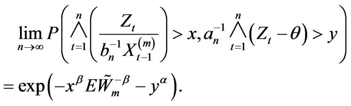
Theorem 2.3. Let denote the stationary AR(1) process such that the innovation distribution satisfies

If then for any we have

where.

Proof. Let us first observe that for

Thus by Lemma 2.9 we obtain

Letting tend to infinity in the above and then tend to 0, we obtain from Lemma 2.5 and that

The theorem now follows from this and Corollary 2.2.

3. Simulation Study

In this section we assess the reliability of our extreme value estimation method through a simulation study. This included a comparison between our estimation procedure and that of three alternative estimation procedures for both the autocorrelation coefficient and the unknown location parameter under two different innovation distributions. Additionally, the degree of approximation for the empirical probabilities of and to its respective limiting distribution was reported.

To study the performance of the estimators

and respectively, we generated 5000 replications for the nonnegative time series for two different sample sizes (500,1000), where is an AR(1) process satisfying the difference equation

The autoregressive parameter is taken to be in the range from 0 to 1 guaranteeing a nonnegative time series and the unknown location parameter is positive when the innovations are taken to be

For this innovation distribution let and be nonnegative constants such that, then this distribution is regularly varying at both endpoints with index of regular variation at infinity and index of regular variation at. For this simulation study two distributions were considered:

Now observe in case i) the innovation distribution is a Pareto distribution with a regular varying tail distribution at with index of regular variation and regular varying at with a fixed index, whereas in case ii) the innovation distribution is regular varying at and with no restriction on or.

First we examine the simulation results for under for each of the six different values considered by computing 5000 estimates using

where and provides the index of the maximal and minimal respectively for, and

where. The means and standard deviations (written below in parentheses), of these estimates are reported in Table 1 along with the average

length for a percent empirical confidence intervals with exact coverage. Since the main purpose of this section is to compare our estimator to Bartlett and McCormick [5] estimator, McCormick and Mathew [2] estimator, and Davis and Resnick’s [13] estimator, the confidence intervals were directly constructed from the empirical distributions of

respectively.

To evaluate and compare the performance of four location estimators, six different scenarios for and are presented in Table 2 under. When, 5000 estimates for each estimator;

, , , and were obtained. The exponent inside the index set

, was set to 0.9.

The means and standard deviations (written below in parentheses), of these estimates are reported in Table 2 along with the average length for a 95 percent empirical confidence intervals. For convenience, the empirical distributions of, ,

, and

were respectively used, where the normalizing constants and are obtained through Equations (3.12)-(3.16) of McCormick and Mathew [2].

Remark. In the case that, converge at

a faster rate than and in the case that, converges at a faster rate than. Lastly, since the McCormick and Mathew [2] paper has the restriction that, only when can the estimators and be fairly compared, whereas only when is our estimator applicable.

Now observe for the selected values being considered, Table 1 shows that our estimator performs at least as well as the three other alternative estimators. This is particularly true under the heavier tail models, i.e. when. In this regime our estimate shows little bias and the average lengths of the confidence intervals are smaller than the other three estimates, sometimes by a wide margin. In particular, when and n = 1000 the confidence interval average length for our method is 3.13, 5.78 and times smaller than the three alternative estimators respectively. This is in part due to the use of one-sided confidence intervals since. Naturally, when, Davis and Resnick least square estimator is more efficient than all three extreme value estimators. While our estimator will always perform slightly better than the

estimator, Bartlett’s and McCormick [5] estimator

main advantage lies with its versatility to perform well for various nonnegative time series, including but not restricted to higher order autoregressive models, along with ARMA models.

Table 2 reveals that our estimator for generally performs better than the three alternative estimators for when. This is particularly true when comparing average confidence interval lengths. Although all three estimators, , and converge to the true value of the parameter as tends to infinity respectively, in this setting they may not compete asymptotically with, say, a conditional least square estimator when. Nonetheless for small sample sizes our simulation study favors over the other three estimators. The difficulty for a least square estimate is that a small negative bias for the estimate of the autocorrelation parameter gives rise to a much larger positive bias in the estimate of. While the affect is not as great, the positive bias found in our estimator and the others for has a significant effect on the estimate for.

Figures 1-4 show a comparison be tween the probability that estimators, , , and are within 0.01 of the true autocorrelation parameter value, respectively. With a sample size of 500, these figures plotted the sample fraction of estimates which fell within a bound of of the true value. Good performance with respect to this measure is reflected in curves near to 1.0 with diminishing good behavior as curves approach 0.0. When, the figures seem to show that our estimator compared to the other three

produced a higher fraction of precise estimates, especially compared to Davis and Resnick estimator. When the regular variation index value is closer to 2, we see a higher fraction of the Davis-Resnick estimates showing better accuracy by this measure. The figures also indicate that McCormick and Mathew’s range estimator produced a consistent high fraction of precise estimates when.

Lastly, we performed a Monte Carlo simulation to study the degree of approximation for the empirical probability, , and to its limiting values, , and respectively. The empirical distributions were calculated from 5000 replications of the nonnegative time series for a sample size of 5000, where

and M was set to 500. Additionally, we restricted. The top two plots in Figure 5 below shows the performance when and the autocorrelation coefficient is for and equal to 0.8, 1.5 respectively. Observe for that the empirical tail probability

mirrors the theoretical probability quite nicely. The lower left plot in Figure 5 displays the asymptotic performance when and the location parameter is for. Notice that the convergence rate of the empirical probability to the theoretical probability is extremely slow. This is not surprising since on average our estimate falls more than 0.1 from the true value when. The lower right plot in Figure 5 displays the asymptotic performance when

for the joint distribution of. Observe that this plot solidifies the asymptotic independence between and.

REFERENCES

- P. J. Brockwell and R. A Davis, “Time Series: Theory and Methods,” 2nd Edition, Springer, New York, 1987.
- W. P. McCormick and G. Mathew, “Estimation for Nonnegative Autoregressive Processes with an Unknown Location Parameter,” Journal of Time Series Analysis, Vol. 14, No. 1, 1993, pp. 71-92. doi:10.1111/j.1467-9892.1993.tb00130.x
- A. E. Raftery, “Estimation Eficace Pour un Processus Autoregressif Exponentiel a Densite Discontinue,” Publications de l’Institut de Statistique de l’Université de Paris, Vol. 25, No. 1, 1980, pp. 65-91.
- R. A. Davis and W. P. McCormick, “Estimation for FirstOrder Autoregressive Processes with Positive or Bounded Innovations,” Stochastic Processes and Their Applications, Vol. 31, No. 1, 1989, pp. 237-250. doi:10.1016/0304-4149(89)90090-2
- A. Bartlett and W. P. McCormick, “Estimation for NonNegative Time Series with Heavy-Tail Innovations,” Journal of Time Series Analysis, 2012. http://onlinelibrary.wiley.com/journal/10.1111/%28ISSN%291467-9892/earlyview
- S. I. Resnick, “Point Processes, Regular Variation and Weak Convergence,” Advances in Applied Probability, Vol. 18, No. 1, 1986, pp. 66-138. doi:10.2307/1427239
- Jiří Anděl, “Non-Negative Autoregressive Processes,” Journal of Time Series Analysis, Vol. 10, No. 1, 1989, pp. 1-11. doi:10.1111/j.1467-9892.1989.tb00011.x
- Jiří Anděl, “Non-Negative Linear Processes,” Applications of Mathematics, Vol. 36, No. 1, 1991, pp. 277-283.
- S. Datta and W. P. McCormick, “Bootstrap Inference for a First-Order Autoregression with Positive Innovations,” Journal of American Statistical Association, Vol. 90, No. 1, 1995, pp. 1289-1300. doi:10.1080/01621459.1995.10476633
- S. I. Resnick, “Heavy-Tail Phenomena: Probabilistic and Statistical Modeling,” Springer, New York, 2007.
- R. A. Davis and S. Resnick, “Limit Theory for Moving Averages of Random Variables with Regularly Varying Tail Probabilities,” Annals of Probability, Vol. 13, No. 1, 1985, pp. 179-195. doi:10.1214/aop/1176993074
- O. Kallenberg, “Random Measures,” Akademie-Verlag, Berlin, 1976.
- R. A. Davis and S. Resnick, “Limit Theory for the Sample Covariance and Correlation Functions of Moving Averages,” Annals of Statistics, Vol. 14, No. 1, 1986, pp. 533-558. doi:10.1214/aos/1176349937