ABSTRACT

We present a new derivation of the Born rule from the assumption of noncontextual probability (NCP). Within the theorem we also demonstrate the continuity of probability with respect to the amplitudes, which has been suggested to be a gap in Zurek’s and Deutsch’s approaches, and we show that NCP is implicitly postulated also in their derivations. Finally, physical motivations of NCP are given based on an invariance principle with respect to a resolution change of measurements and with respect to the principle of no-faster-than-light signalling.

1. Introduction

The fundamental probabilistic postulate which allows QM its successful predictions was first introduced by Born (from a suggestion by Einstein) in 1926 within the scattering theory [1]. The question if such postulate could be derived as a theorem from other postulates of QM was quickly posed. A first answer was provided by Von Neumann and included in his famous book of 1932 on the mathematical foundations of QM [2]. His theorem nowadays does not enjoy much attention since it is believed to contain more assumptions than Gleason’s [3,4]. Different attempts have been discussed in the context of the relative-state [5] and the many-worlds interpretations [6] of QM by Finkelstein [7] and Hartle [8], which have analyzed an endless sequence of measurements to show that the relative frequency follows the Born rule. However, the meaning in the real world of an infinite sequence of measurements is controversial and it is doubtful whether these proofs contain circularities [9-14].

The 1957 Gleason work [4] is regarded as the most important derivation of the Born rule [15], but this theorem is usually considered quite formal and difficult to grasp. Moreover, it is based on the concept of noncontextual probability (NCP), whose connection with physics is not clear. In the structure of the Gleason theorem, every Hilbert subspace corresponds to an observable quantity. Each one of such subspaces is representable by a projection operator. A projector can represent the question with answer yes or not concerning an experiment testing whether the system has the respective state. A complete set of mutually commuting projectors corresponds to a set of questions which can simultaneously be asked in a measurement. In the logical-algebraic approach [16], probability is a measure defined over a projection lattice (set of closed subspaces) of Hilbert space, a mapping. The postulates on which the theorem rests are:

1) The probability assigned to a complete set of projectors is normalized:

(1)

2) For any sequence of mutually orthogonal projectors:

(2)

Assuming Postulate 2) is equivalent to postulating NCP for projective measurements (or, i.e., according to the definition by Spekkens, measurement noncontextuality [17]): the probability of a certain occurrence, for example the answer yes for a projector, does not depend on other questions simultaneously tested, that is, on other projectors. In terms of basis vectors, the probability of obtaining a given state is independent of the basis it belongs to. To illustrate this important point, let us consider, for instance, two complete set of mutually orthogonal projectors, with, where. From the normalization postulate of probability:

(3)

(4)

where in principle and may be different. In the subspace orthogonal to we have

, then

and from Postulate 2:

(5)

Then, by comparing Equation (3) and Equation (4), we get. It is also possible to show the vice versa, i.e, if NCP holds then Postulate 2 is true.

From Postulates 1 and 2 it follows Gleason’s Theorem: For a Hilbert space with dimension there exists a density operator which acts on such that the probability measure for every projector is the trace rule:

(6)

namely, the Born rule.

More recently, new proofs appeared in the literature with the intention of being “more physically motivated than the theorem of Gleason” [18]. Their aim, as the ours in the present work, is to shed new light on the physical principles of QM, particularly on the origin of the Born rule. Indeed, Gleason’s theorem gives “rather little insight into the emergence of quantum probabilities and the Born rule” [19].

Particularly interesting are Deutsch’s and Zurek’s derivations [18,20-25]. Their approaches to the Born rule have similar structures. As a first step, they use an invariance principle in order to show that equal amplitudes correspond to equal probabilities. Deutsch finds such principle in the theory of decisions (for critical discussions and further elaborations see [26-28]). Zurek introduces an environment-assisted invariance principle [29,30], envariance, in the framework of a relative-state approach where the system under measurement jointly evolves with the environment and, possibly, with one or more auxiliary measurement devices. After demonstrating the correspondence between equal amplitudes and equal probabilities, both Zurek and Deutsch consider a finegraining technique to deal with the general case of different amplitudes of the initial state. For this purpose they have to introduce auxiliary systems which become entangled with.

However, fine-graining has been questioned: Caves [23] considers disturbing the necessity of introducing additional systems of adequate dimensions, possibly in an infinite Hilbert space, in order to reach the wanted approximation to irrational probabilities. Barnum [25] points out an even more stringent weakness: the step from rational to irrational amplitudes requires the continuity of the probability with respect to such amplitudes and such a property is not demonstrated by Zurek and Deutsch. We note that a fundamental and extensive part of Gleason’s theorem is actually devoted to prove that the probability is continuous. For several other controversial points of Zurek’s demonstration, the most of them shares with Deutsch’s, we refer to [19,23-25].

So, although Gleason-type theorems are usually considered well established, a simple, physically justified and shared derivation of the Born rule is not yet present in the literature. With our work we intend to fill this gap.

In the next section we propose a new derivation of the Born rule from the NCP assumption for projective measurements and pure states, the generalization to mixed states being immediate. Whereas Gleason assumes that a density operator acting on describes a general quantum state of the system only at the final step of his work, we introduce vectors of the Hilbert space describing quantum states from the very beginning of our derivation. On the one hand it allows a much more elementary deduction of the Born rule, and on the other hand it makes the postulates and the physical principles of our theorem easier to analyze in comparison with the previous demonstrations. Moreover, involving Zurek’s and Deutsch’s demonstrations pure states, also the connections between those works, the Gleason Theorem and the ours are clearer.

We do not enter into the controversy about the origin and the meaning of probability, and following Gleason and others (see also Mohrhoff in [24]), we assume the existence of probability defined on a quantum state. In addition, differently by Zurek, we do not suppose unitary evolution and consider a single system. As Gleason’s Theorem, our result holds for a Hilbert space with, whereas in general, because of fine-graining, Zurek’s and Deutsch’s hold for. We also give a rather simple derivation that the probability is continuous from NCP. Without this proof, Deutch’s and Zurek’s results only hold for rational values of amplitudes.

In Section III we generalize our theorem to include entangled states and multi-particles systems. Since the Hilbert space of such systems has dimension which is the product of the dimensions of its components, the coupling of a subsystem with with another subsystem with enables us to extend the Born rule also to such space.

In Section IV we show that the Gleason postulate of NCP occurs in the use of fine-graining and that such a postulate is a hidden assumption of Zurek’s and Deutsch’s proofs. Indeed, fine-graining is a resolution change of our measurements and NCP is equivalent to a condition of invariance with respect to such a change: finegraining on a subspace of the state must not alter the probability of finding the system in a different subspace. This resolution invariance is an intuitive and physically natural interpretation of measurement noncontextuality.

Finally, in Section V, we show that the condition of noncontextual probability, or resolution invariance, can also be deduced by the hypothesis of no-faster-than-light signalling of the Special Relativity.

2. Born Rule as a Theorem from Noncontextual Probability

Contrarily to the principles of classical mechanics, the axioms of QM do not have an equally shared and clear formulation. We do not want to enter into such a thorny issue, related to the interpretative problems of QM. For our purpose, from the quantum postulates generally considered in standard presentations of QM (see, e.g., [31-34]), we can extract the following common assumptions:

Postulate I:

At the time the state of every physical system is described by a normalized vector belonging to a Hilbert space.

Postulate II:

Every measurable physical quantity is described by a Hermitian operator acting in.

Postulate III:

The only possible result of a measurement of an observable is one of the eigenvalues of, (as the customary habit, from now on we will identify the observable with its operator).

Postulate IV:

If the measurement of the observable on the system in the state gives the result, the state of the system immediately after the measurement is the associate normalized eigenstate (non-degenerate case).

Postulate I is known as the Completeness Postulate of QM. Postulate II links an observable quantity with an operator in a Hilbert space (observable-operator link). Postulate III connects a particular value of that observable with an eigenvalue of the corresponding operator (value-eigenvalue link). Postulate IV relates a detected eigenvalue with the state of the system (eigenvalueeigenstate link).

Now consider a Hermitian observable with discrete eigenvalues and eigenstates, , and a single system described by the state. is a complete orthonormal set and can be decomposed into components:

(7)

We intend to prove the following

Theorem 1:

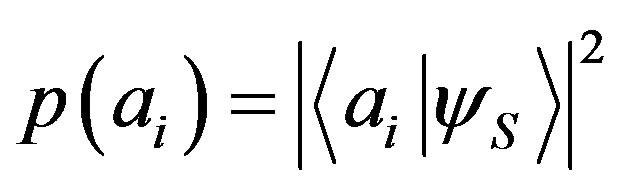
If NCP and Postulates I-IV hold, then for the probability of obtaining the non-degenerate eigenvalue, measuring on the state, is necessarily given by the square modulus of the inner product:

(8)

where is the eigenstate associated with the eigenvalue.

We assume the probability as a primitive concept and we begin the derivation of Theorem 1 by proving some simple lemmas. We underline that any theorem having the aim to prove the Born rule has to face the fact that the connection between probability and quantum state must be postulated or deduced by other means. Gleason, for instance, postulates the probability to be a measure defined on states of the basis. As Gleason, we suppose QM to be a probabilistic theory, which makes predictions about probabilities of occurrences of observable quantities, and that probabilities are functions of quantum states. Then, from QM postulates we want to show that

Lemma 1:

The probability of obtaining an eigenvalue is equal to the probability of obtaining the respective eigenstate (statistical case):

(9)

wang#title3_4:spProof:

Suppose that the system is prepared with the eigenvalue, in this case. According to Postulate IV if then, and vice versa. But correspond to mutually exclusive events, thus has to be for. Then must necessarily be too, since, otherwise, having obtained with a measurement the state we should assign to the system the eigenvalue, in contradiction with the exclusivity property of events. Therefore we have the equations for the conditional probabilities for a non-statistical case:

(10)

which represent the probability of finding the state for systems prepared with certainty with eigenvalue, and vice versa. Because of Postulate III, the only possible result of a measurement is one of the eigenvalues of. Consider then a generic preparation of the initial state with. Introducing the joint probability and considering the general validity of the Bayesian formula for the joint probabilities, we have

(11)

where we have used Equation (10) in the conditional probabilities of Equation (11).

We note from Equations (10) and (11) that

and that represent a set of complete and mutually exclusive events:

(12)

Lemma 1 can be easily generalized for entangled states as well. For instance, consider the state:

(13)

where is a new observable commuting with, with eigenvalues and eigenstates, , and, (we point out that does not necessarily have to belong to another system: for example, could be the spin observable and the position observable of one particle). Consider the pairs of eigenvalues, and eigenstates. By using conditional probabilities, it follows that on the generic state:

(14)

(see Appendix A for a proof of this). Then the probability is again given by:

(15)

With a similar reasoning we can also show that. We notice from Equations (14) and (15) that the outcomes of are mutually exclusive events as well, with the condition of normalization following from the normalization of.

Lemma 2: If a coefficient of an eigenstate in Equation (7) is zero, the probability of obtaining the corresponding eigenvalue and eigenstate is zero as well.

Proof: If, for instance, , the corresponding state will be orthogonal to. We can think as eigenstates of the projector

with eigenvalues. The Hermitian operator represents the observable testing whether the system is prepared with the state or not.

The pair is a complete orthonormal basis of a subspace of.

With the system prepared in the state:

. From Lemma 1, it follows that

and because eigenvalues are exclusive events. So, if we apply Lemma 1 again to the previous equation, considering that is eigenstate of both and, we have

and.

Also Lemma 2 can be directly generalized to entangled states. For instance, if in the state the coefficient then. In particular, if the state of the system is in a Schmidt decomposition:

(16)

from Lemma 1 and Lemma 2, since for, it follows the perfect correlation property:

(17)

Lemma 3:

If the measurement is noncontextual then the probability of obtaining the eigenvalue can only depend on the modulus of the coefficient:

(18)

wang#title3_4:spProof:

Let us recall the meaning of NCP with an example (we refer to the work by Spekkens for an extensive analysis of the contextuality concept in arbitrary operational theories and in QM [17]). Consider two operators and which do not commute, []0, in a Hilbert space with. Eigenvalues and eigenstates of and are, respectively:

(19)

where they have in common the eigenvalue and the associate eigenstate (we see that this is possible, if and must not commute, just for). We can write the state in the two different bases of Equation (19):

(20)

In general, the probability of obtaining the eigenvalue could depend on whether we measure the observable or. In other words, the probability could be different if we were in the experimental context which is prepared for measuring which value assumes of the triplet or which value assumes of the triple.

With the result of Lemma 1 and the completeness postulate of QM, we can write the more general probability in different experimental contexts as:

(21)

The probability is noncontextual, and we have measurement noncontextuality, if does not depend on the measurement with other eigenvalues:

(22)

or, according to Lemma 1, the probability does not depend on the measurement with other eigenstates:

(23)

Then, by assuming NCP, Equations (21) can be reduced to the equation:

(24)

stating that the probability only depends on the eigenstate and, from the completeness postulate of QM and NCP, on the state of the system.

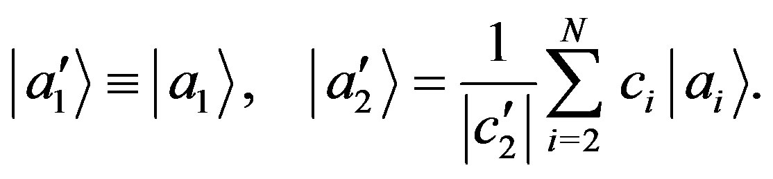
Thus, let us choose a new basis such that the state in Equation (7) is written with only two components:

(25)

where for, is the modulus of the amplitude and

(26)

could be regarded as eigenstates of an observable with eigenvalues checking whether our system is in the state or not.

According to NCP the transformation of basis of the state cannot change the probability:

(27)

Now we expressly write the phase of the coefficient in the state of Equation (25):

(28)

We get for the state the probability:

(29)

Therefore, considering the normalization and that the components of the orthonormal basis are the constants, the most general function of the probability in Equation (29) can be written as:

(30)

A similar argument when applied to every state gives

(31)

However, by using the conservation of probability we can show the independence from the phase of. Indeed, let us suppose to have two different states and which are distinct just with respect to the phase of the component (to simplify the notation, we select a basis such that the components of the states are different from zero only in a subspace with):

(32)

where with we have denoted the new phase. The conservation of the probability requires:

(33)

where from Lemma 2 we have used the fact that if. Thanks to Equation (31), we have that

(34)

From this and Equation (33), we also get:

(35)

which is equivalent to write:

(36)

Therefore, since is an arbitrary phase, the probability does not depend on it but can only depend on the modulus. So, we can set, and this proves our lemma (the generalization to probabilities of other eigenvalues is immediate).

Now we have all the ingredients to prove our

Theorem 1:

the probability is given by the square modulus of coefficient.

Proof:

Let us consider the state with in Equations (7). For the sake of simplicity we focus our attention again on. We choose two bases and such that

(37)

(38)

where for, for and. From the conservation of the total probability for the states of the two different bases we get respectively:

(39)

(40)

where from NCP we have the same probability in both Equations (39) and (40). With a change of variable we can write Equation (18) as. From Equations (39) and (40) it follows that

(41)

By comparing the two Equations (41) we get:

(42)

Since the state is normalized, we also have

(43)

(44)

and

(45)

Putting this in Equation (42):

(46)

Now we recall that a function is linear with respect to the variable if and only if the two following properties are jointly satisfied:

(47)

where is any real number. We remark that if is a rational number, it can be shown that the homogeneity follows from the additivity. Furthermore, since rational numbers form a subset dense in the set of real numbers, such derivation can be extended to the case of irrational, if is a continuous function [35].

Therefore, the condition of additivity is sufficient to establish the linearity if is a continuous function. On the contrary, if is not assumed to be continuous, the condition of additivity implies linearity only for rational values of the variable.

Hence, if we assume that the probability is continuous with respect to the coefficients, Equation (46) is a constraint of linearity for the probability. In this case we can write:

(48)

where denotes a constant. From Lemma 1 we have that and therefore and. Hence, the Born rule is deduced for continuous probabilities.

We point out that we have postulated the continuity of probability. However, a derivation of such a property from noncontextuality is present in Gleason’s work and it occupies a prominent part of that paper. Therefore in comparison to Gleason we have only accomplished half the job: as Bertrand Russell once said, postulating is equivalent to theft on the honest fatigue. On the other hand, if the continuity of probability is neither postulated nor demonstrated, we can only say that the Born rule applies only for rational values of the coefficients.

Thus we now intend to complete our derivation by showing from NCP that the probability is continuous and that the Born rule also holds for irrational coefficients.

Consider, once again,. We select a basis

such that the state is written with two components as in Equation (38), with, and the conservation of probability is given by Equation (40).

Then we choose a new basis in general with, for, but with so that we can write

(49)

The conservation of probability for the new states of the basis requires that

(50)

From the previous condition we have the inequality:

(51)

By comparing Equation (40) with Equation (51) and since, thanks to NCP, the probability is the same in these equations, we get

(52)

Finally, we choose a third basis such that for, this time with:

(53)

The conservation of probability gives us:

(54)

From Equation (54) we get the inequality:

(55)

Therefore the probability is in the range:

(56)

Suppose to be an irrational number, we choose rational values for and so that and. By putting, Equation (56) becomes

(57)

with. Let us denote with the orthonormal state to. Consider the limits,

and,. From Equation (38) we have, and,. Summarizing, with the normalization condition in Equation (44) we get:

(58)

Because rational numbers form a dense set in the set of real numbers, we can always find a couple of numbers which are as near as we want to the irrational number. Therefore, from Equation (57) it follows that the oscillation of the function is zero at. Consequently, the probability must be continuous at and even if.

3. Noncontextual Probability for Entangled States

Theorem 1 with NCP can be generalized to include also entangled states, bipartite or multipartite systems and quantum measurement devices.

Let us indicate with the context, including our experimental devices and the environment, and with its possible states. Consider again the measurement of the two observables and introduced in the proof of Lemma 3 in the previous section. The choice of measuring either the eigenvalues or together with corresponds to two different experimental arrangements and.

Suppose that at time the system is in the initial state. At time, after the interaction with the measurement device, the entanglement between the system with the experimental setup correlates the observable (or) of the system with the pointers of the experimental device. If we measure we have the state:

(59)

while if we measure we get:

(60)

The global wave functions Equations (59) and (60) are different in the different contexts and. So the two probabilities

(61)

may be different. The possible contextuality of probability is now included inside the description of the global system of the quantum state. We notice that it is no longer possible to write

(62)

if we accept the completeness of QM. Otherwise, indeed, some parameters would be outside the description of the state, which now englobes not only the system but also the context of the measurement. This should imply the existence of hidden variables.

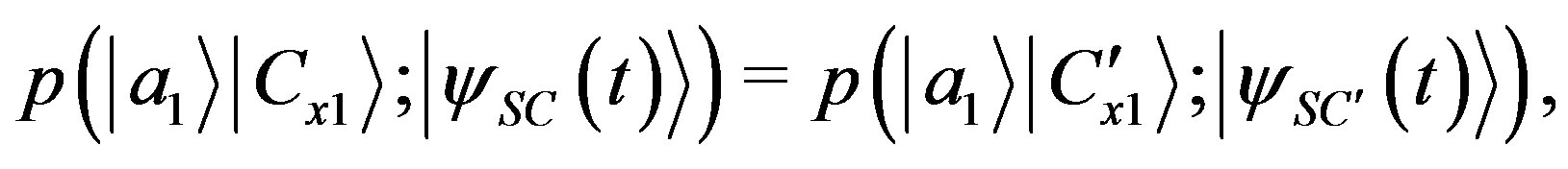
Assuming NCP requires the equality between the probabilities in Equation (61):

(63)

which generalizes the condition in Equation (23). In fact, Equation (63), by the perfect correlation property of Equation (17), becomes equivalent to Equation (23).

In a similar way as in the previous derivation, by using the state of Equation (59) and a state with a new basis such that for, we can write:

(64)

From the condition of NCP it is not difficult to deduce that must hold. Then, employing states like in Equation (59) and Equation (64) and from NCP, normalization condition and conservation of probability, it is possible to prove again the linearity of the probabilities with respect to the square moduli of the amplitudes (continuity can also be generalized to the present case). Putting all pieces together, we get

(65)

We note that the state of the global system is in the Hilbert space with dimension. If this allows us to include in the derivation of the Born rule also states with. In fact, consider a system described by a state in a Hilbert space with and basis. With a measurement we could use the context as an ancilla system to build the following entangled states:

(66)

where is obtained by dividing the part of the state associated with the eigenvalue into two regions. So it is possible to demonstrate that

as in the previous cases. We note that the condition for the state of the ancilla system coupled with is necessary to obtain, from Equations (66) by the NCP property of Equation (63), a constraint of additivity and linearity similar to that which is at Equations (39)-(46).

4. Noncontextual Probability and Resolution of the Measurement

A simple application of Lemma 3 shows that equal amplitudes are related to equal probabilities, i.e: if with then. Whereas Lemma 3 is derived from the NCP principle, the same result was obtained by Zurek and Deutsch on the base of two different invariance principles. Then both authors study the more general case with states having different rational amplitudes using the fine-graining technique. We shortly summarize their results. We consider the fine-graining in Zurek’s approach with the environment in a simple situation (our remarks also hold for Deutsch’s similar derivation). We assume that the state of the system is in a Hilbert space with, entangled with the state of the environment such that their joint state is

(67)

The idea is to transform this state with unequal coefficients into a state with equal coefficients by fine-graining. This goal is reached by extracting from the environment an ancilla system having states

(68)

which become correlated with the states of. Within a quantum measurement, can be regarded as a counter and as a new orthonormal basis of pointer states. Denoting with the new states of the environment without, after the interaction between and we have the joint system

(69)

which can be expressed with the new basis of pointer states of Equation (68):

(70)

Now we have a new state with equal amplitudes. But how can we be sure that after fine-graining the probability with the state is the same with the state or? In principle they could be different, so to legitimately use the fine-graining reasoning we have to assume the equality:

(71)

equivalent to the condition of NCP encountered in Equation (63) of Section 3. Then, in their derivations Zurek and Deutsch implicitly assume NCP. We notice that fine-graining is equivalent to a change of measurement resolution, and this has been used in our derivation as well. A change of resolution, for instance, is considered going from Equation (39) to Equation (40). There we assumed from NCP that is the same in the two equations and therefore:

(72)

where is the probability of finding the state of the system in the subspace orthonormal to, whereas and are the probabilities of finding it, respectively, in the subspaces and of the subspace orthonormal to. In fact, in terms of projectors, Equation (72) can be written as Gleason’s Postulate 2:

(73)

Thus NCP could be physically interpreted as a probability invariance when we change the resolution of the measurement connected with other properties of the system. This interpretation gives physical insight to the NCP principle as an invariance under changing resolution. The probability of one measurement outcome should not change if we make coarse or fine-graining over other measurement outcomes. We point out that coarse/fine graining could be done through a post-processing after the first measurement. Therefore, NCP is a natural assumption if we do not want signalling from the future to the past.

5. Noncontextual Probability and No-Faster-than-Light Signalling

In general, every measurement in the real world happens in the spacetime. Every measurement of any observable is necessarily reduced to a measurement of position at a certain time. For instance, the Stern-Gerlach apparatus correlates a spin observable with a position observable so that different values of the spin univocally correspond to different position values of the system. A measurement of position detects the spin value of the system.

Let us introduce in our representation of the observable position. We assume that at time, the system is in the initial state. For simplicity of notation, from now on we denote with the position state of the system with its context, where the letter will remind us the dependence on the position of the system and the experimental apparatus. Suppose that we can measure either the values of the observable or the values of the observable. In the context of measurement we get:

(74)

while for the experimental context we have the different state:

(75)

We want to prove the following

Theorem 2:

If we assume the no-faster-than-light signalling condition for measurement events which are spacelike separate, then the probability must be noncontextual.

Proof:

Consider a set of identically prepared systems in the initial state. In order to estimate the probabilities and

, let us assume that our experimental device is arranged to measure how many systems have the eigenvalue at the point and the eigenvalues (Equation (74)) or the eigenvalues (Equation (75)) at the points and. This could be done by first dividing the systems in two parts, one associated with the state at the point and an other one associated with the orthogonal state at a different point (see the superposition state in Equation (78)), then by dividing such a state in two sub-parts, associated either with the basis, or with the basis at the points, , respectively connected with the states in Equations (74)-(75).

If the measurements of or at the points and are events spacelike separate with respect to the measurement of at, according to the relativistic hypothesis of no-signalling, the probability of getting the eigenvalue has to be the same in both different experimental contexts and. Otherwise an observer situated in the place of measurement of or would be able to send a superluminal signal to another observer situated in the place where is measured. Then, according to the no-faster-than-light signalling hypothesis:

(76)

which is to say, with the result of Equation (17):

(77)

Therefore must be noncontextual.

Consider, beside the measurement of the eigenvalues of the observable, also the simple possibility of measuring whether our systems assume the eigenvalue or not, which is equivalent to check whether the systems are in the state or in the subspace orthogonal to it. In such a case, during the process of measurement, the systems will be in the state:

(78)

If the two choices of measuring either or correspond to events spacelike separate, as mentioned above, from the condition of no-signalling we must have the NCP condition:

(79)

From Equation (79) the conservation of probability imposes also the equation:

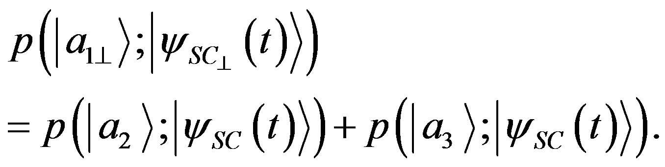(80)

As we showed at the end of Section IV, Equation (80) is equivalent to the initial hypothesis adopted by Gleason. Moreover, by examining Equation (79) we understand that it is analogous to assuming an invariance condition of the probability under a resolution change of our measurement, or fine/coarse graining. So, at least for spacelike separate measurements, NCP could be deduced by a relativistic principle. However, the Born rule holds for general events, not only for spacelike separate ones. Hence NCP or, equivalently, the invariance of probability when we change resolution, seem to be more general principles.

6. Concluding Remarks

We have given a new derivation of the Born rule based on the noncontextuality for projective measurements and on some non-statistical postulates of QM. The introduction of a pure quantum state of the system has allowed a more elementary proof than Gleason’s theorem. This may seem, at first sight, a loss of generality with respect to Gleason’s proof, however Gleason also introduces vectors of basis which can be regarded as states of the system. Moreover, the step from pure states to density operators and to the trace rule for mixed ensembles is quite natural when we already have the Born rule [36].

As in Gleason’s, our derivation holds for, where could be finite or infinite. The origin of this dimensional limitation lies in the fact that for the same state vector may belong to several distinct orthonormal bases. This, with NCP, the normalization of the probability and the quantum state, brings us to a constraint of functional linearity between the probability and the amplitude square modulus. Our theorem can be simply generalized in order to include multipartite states. In such a case, if a part of the global system has, the Born rule can also be proved to hold in subspaces with.

We have also given a derivation that the probability is continuous with respect to the amplitudes using measurement noncontextuality. This fills a gap of Zurek’s and Deutsch’s demonstrations.

Physical motivation for NCP could come from a relativistic principle of no-faster-than-light signalling. However, the Born rule also holds for measurements which are non-spacelike separate, hence NCP seems to be a more fundamental principle. Finally, we have given an interpretation of measurement noncontextuality as an invariance of the probability under a resolution change of our measurement.

7. Acknowledgements

This work has been supported by the EU-STREP Project QIBEC within the activities of the BEC center. QSTAR is the MPQ, IIT, LENS, UniFi joint center for Quantum Science and Technology in Arcetri.

REFERENCES

Appendix A

We want to generalize the result of Lemma 1 for entangled states. Suppose that the system is prepared with eigenvalues and therefore with eigenstates. Similarly to the unentangled case, we can deduce that if and only if. This relation, translated into conditional probabilities, is equivalent to writing:

(81)

Then, from Equation (81) we have that for a generic state as in Equation (13):

(82)

If the observable has an eigenstate and the observable has an eigenstate then the tensorial product is an eigenstate of the observable, and vice versa. The eigenstates

of form a basis of Hilbert space

.

If we indicate with the probability of obtaining the eigenstate, with a measurement of, we have if and only if, or, in equivalence:

(83)

From Equations (82)-(83), through the use of the conditional probabilities, it immediately follows that on the state we have.

NOTES

^*Corresponding author.

REFERENCES

- J. A. Wheeler and W. H. Zurek, Eds., “Quantum Theory and Measurement,” Princeton University Press, Princeton, 1963.
- J. von Neumann, “Mathematical Foundations of Quantum Mechanics,” Princeton University Press, Princeton, 1955. doi:10.1063/1.3061789
- T. F. Jordan, “Linear Operators for Quantum Mechanics,” John Wiley Sons, New York, 1969. doi:10.1119/1.1975255
- A. M. Gleason, “Measures on the Closed Subspaces of a Hilbert Space,” Journal of Mathematics and Mechanics, Vol. 6, No. 6, 1957, pp. 885-893.
- H. Everett, “Relative State Formulation of Quantum Mechanics,” Reviews of Modern Physics, Vol. 29, No. 3, 1957, pp. 454-462. doi:10.1103/RevModPhys.29.454
- B. S. DeWitt, “The Many-Universes Interpretation of Quantum Mechanics,” In: B. d’Espagnat, Ed., Foundations of Quantum Mechanics, Academic Press, New York, 1971.
- D. Finkelstein, “The Logic of Quantum Mechanics,” Transactions of the New York Academy of Sciences, Vol. 25, No. 6, 1965, pp. 621-637. doi:10.1111/j.2164-0947.1963.tb01483.x
- J. B. Hartle, “Quantum Mechanics of Individual Systems,” American Journal of Physics, Vol. 36, No. 8, 1968, pp. 704-712. doi:10.1119/1.1975096
- N. Graham, “The Measurement of Relative Frequency,” In: B. S. DeWitt and N. Graham, Eds., The Many-Worlds Interpretation of Quantum Mechanics, Princeton University Press, Princeton, 1973.
- R. Geroch, “The Everett Interpretation,” Noûs, Vol. 18, No. 4, 1984, pp. 617-633. doi:10.2307/2214880
- E. Farhi, J. Goldstone and S. Gutmann, “How Probability Arises in Quantum Mechanics,” Annals of Physics, Vol. 192, No. 2, 1989, pp. 368-382. doi:10.1016/0003-4916(89)90141-3
- H. Stein, “The Everett Interpretation of Quantum Mechanics: Many Worlds or None?” Noûs, Vol. 18, No. 4, 1984, pp. 635-652. doi:10.2307/2214881
- A. Kent, “Against Many-Worlds Interpretations,” International Journal of Modern Physics A, Vol. 5, No. 9, 1990, pp. 1745-1762. doi:10.1142/S0217751X90000805
- T. Endo, “Verification of Born’s Rule by a Quantum Mechanical Meter,” Physics Letters A, Vol. 308, No. 4, 2003, pp. 256-258. doi:10.1016/S0375-9601(03)00083-5
- C M. Caves, C. A. Fuchs and R. Schack, “Quantum Probabilities as Bayesian Probabilities,” Physical Review A, Vol. 65, No. 2, 2002, pp. 1-6. doi:10.1103/PhysRevA.65.022305
- M. Redhead, “Incompleteness, Nonlocality and Realism,” Claredon Press, Oxford, 1989. doi:10.1119/1.16032
- R. W. Spekkens, “Contextuality for Preparations, Transformations, and Unsharp Measurements,” Physical Review A, Vol. 71, No. 5, 2005, pp. 1-17. doi:10.1103/PhysRevA.71.052108
- W. H. Zurek, “Environment-Assisted Invariance, Entanglement, and Probabilities in Quantum Physics,” Physical Review Letters, Vol. 90, No. 12, 2003, pp. 1-4. doi:10.1103/PhysRevLett.90.120404
- M. Schlosshauer and A. Fine, “On Zurek’s Derivation of the Born Rule,” Foundations of Physics, Vol. 35, No. 197, 2005, pp. 197-213. doi:10.1007/s10701-004-1941-6
- D. Deutsch, “Quantum Theory of Probability and Decisions,” Proceedings of the Royal Society of London A, Vol. 455, No. 1988, 1999, pp. 3129-3137. doi:10.1098/rspa.1999.0443
- W. H. Zurek, “Probabilities from Entanglement, Born’s Rule from Envariance,” Physical Review A, Vol. 71, 2005, pp. 1-29. doi:10.1103/PhysRevA.71.052105
- W. H. Zurek, “Entanglement Symmetry, Amplitudes, and Probabilities: Inverting Born’s Rule,” Physical Review Letters, Vol. 106, No. 25, 2011, pp 1-4. doi:10.1103/PhysRevLett.106.250402
- C. M. Caves, “Notes on Zurek’s Derivation of the Quantum Probability Rule,” 2005. http://info.phys.unm.edu/caves/reports/ZurekBornderivation.pdf
- U. Mohrhoff, “Probabilities from Envariance?” International Journal of Quantum Information, Vol. 2, No. 2, 2004, pp. 221-230. doi:10.1142/S0219749904000195
- H. Barnum, “No-Signalling-Based Version of Zurek’s Derivation of Quantum Probabilities: A Note on Environment-Assisted Invariance, Entanglement, and Probabilities in Quantum Physics,” 2003. arXiv: quant-ph/0312150
- H. Barnum, C. M. Caves, J. Finkelstein, C. A. Fuchs and R. Schack, “Quantum Probability from Decision Theory?” Proceedings of the Royal Society of London A, Vol. 456, No. 1997, 2000, pp. 1175-1182. doi:10.1098/rspa.2000.0557
- S. Saunders, “Derivation of the Born Rule from Operational Assumptions,” Proceedings of the Royal Society of London A, Vol. 460, No. 2046, 2004, pp. 1-18. doi:10.1098/rspa.2003.1230
- D. Wallace, “Everettian Rationality: Defending Deutsch’s approach to probability in the Everett interpretation,” Studies in History and Philosophy of Modern Physics, Vol. 34, No. 3, 2003, pp. 415-438. doi:10.1016/S1355-2198(03)00036-4
- W. H. Zurek, “Decoherence, Einselection, and the Quantum Origins of the Classical,” Reviews of Moder Physics, Vol. 75, No. 3, 2003, pp. 715-775. doi:10.1103/RevModPhys.75.715
- W. H. Zurek, “Quantum Darwinism and Envariance,” 2003. arXiv: quant-ph/0308163
- C. Cohen-Tannoudji, B. Diu and F. Laloë, “Quantum Mechanics,” Hermann and Wiley, Paris, 1977.
- N. Zettili, “Quantum Mechanics, Concepts and Applications,” Wiley, Chichester, 2001.
- W. Greiner, “Quantum Mechanics, An Introduction,” Springer-Verlag, Berlin, 2000.
- A. Galindo and P. Pascual, “Quantum Mechanics I,” Springer-Verlag, Berlin, 1990. doi:10.1007/978-3-642-83854-5_2
- M. Kuczma, “An Introduction to the Theory of Functional Equations and Inequalities,” Birkhäuser, Basel, 2009. doi:10.1007/978-3-7643-8749-5
- J. J. Sakurai, “Modern Quantum Mechanics,” Addison-Wesley, San Francisco, 1994.