ABSTRACT

In this paper, a two-parameter Lindley distribution, of which the one parameter Lindley distribution (LD) is a particular case, for modeling waiting and survival times data has been introduced. Its moments, failure rate function, mean residual life function, and stochastic orderings have been discussed. It is found that the expressions for failure rate function mean residual life function and stochastic orderings of the two-parameter LD shows flexibility over one-parameter LD and exponential distribution. The maximum likelihood method and the method of moments have been discussed for estimating its parameters. The distribution has been fitted to some data-sets relating to waiting times and survival times to test its goodness of fit to which earlier the one parameter LD has been fitted by others and it is found that to almost all these data-sets the two parameter LD distribution provides closer fits than those by the one parameter LD.

1. Introduction

D. V. Lindley [1,2] introduced a one-parameter distribution, known as Lindley distribution, given by its probability density function

(1.1)

It can be seen that this distribution is a mixture of exponentialand gamma distributions. Its cumulative distribution function has been obtained as

(1.2)

M.E. Ghitany, B. Atieh, and H. Nadarajah [3] have discussed various properties of this distribution and showed that in many ways (1.1) provides a better model for waiting times and survival times data than the exponential distribution. The first four moments about origin of the one-parameter LD have been obtained as

(1.3)

and its central moments have been obtained as

(1.4)

A discrete version of this distribution has been suggested by F. G. Deniz and E. C. Ojeda [4] having its applications in count data related to insurance. M. Sankaran [5] obtained the Lindley mixture of Poisson distribution. J. Mazucheli and J. A. Achcar [6], M. E.Ghitany, F. Alquallaf, D. K. Al-Mutairi and H. A. Hussain [7], Bakouchi et al [8] are some among others who discussed its various applications.

In this paper, a two parameter Lindley distribution, of which the one-parameter LD (1.1) is a particular case, for modeling waiting and survival times data has been suggested. Its first four moments and some of the related measures have been obtained. Its failure rate function, mean residual life function and stochastic orderings have also been studied. Estimation of its parameters has been discussed and the distribution has been fitted to some of those data-sets where the one-parameter LD has earlier been fitted by others relating to waiting times and survival times data, to test its goodness of fit.

2. A Two-Parameter Lindley Distribution

A two-parameter Lindley distribution (Two-parameter LD) with parameters and is defined by its probability density function (p.d.f.)

(2.1)

It can easily be seen that at, the distribution (2.1) reduces to the one parameter LD (1.1) and at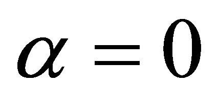, it reduces to the exponential distribution with parameters. The p.d.f. (2.1) can be shown as a mixture of exponential and gamma distributions as follows:

(2.2)

where

and.

The first derivative of (2.1) is obtained as

and so

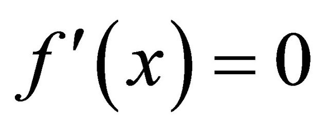gives.

From this it follows that1) for is the unique critical point at which is maximum.

2) for, 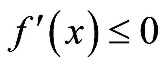i.e. 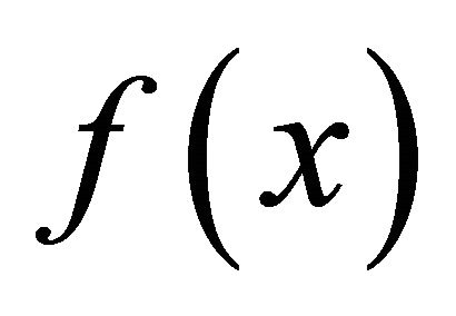is decreasing in.

Therefore, the mode of the distribution is given by

(2.3)

The cumulative distribution function (c.d.f) of the twoparameter LD is given by

(2.4)

3. Moments and Related Measures

The rth moment about origin of the two-parameter LD has been obtained as

(3.1)

Taking and 4 in (3.1), the first four moments about origin are obtained as

(3.2)

It can be easily verified that for, the moments about origin of the two-parameter LD reduce to the respective moments of the one parameter LD. Further, since the mean of the distribution is always greater than the mode, the distribution is positively skewed. The central moments of this distribution have thus been obtained as

(3.3)

(3.4)

It can be easily verified that for, the central moments of the two-parameter LD reduce to the respective moments of the one parameter LD.

The coefficients of variation, skewness

and the kurtosis of the two-parameter LD are given by

(3.6)

(3.7)

(3.5)

(3.8)

It can be easily verified that for, the coefficients of variation, skewness, and the kurtosis of the two-parameter LD reduce to the respective coefficients of the one parameter LD.

4. Failure Rate and Mean Residual Life

For a continuous distribution with p.d.f. and c.d.f.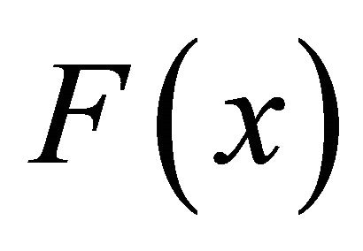, the failure rate function (also known as the hazard rate function) and the mean residual life function are respectively defined as

(4.1)

and

(4.2)

The corresponding failure rate function, and the mean residual life function, of two-parameter LD are thus given by

(4.3)

and

(4.4)

It can be easily verified that and. It is also obvious that

is an increasing function of and, whereas is a decreasing function of and, and increasing function of. For, (4.3) and (4.4) reduces to the corresponding measures of the one parameter LD. The failure rate function and the mean residual life function of the distribution show its flexibility over one parameter LD and exponential distribution.

5. Stochastic Orderings

Stochastic ordering of positive continuous random variables is an important tool for judging the comparative behaviour. A random variable is said to be smaller than a random variable in the 1) stochastic order if for all;

2) hazard rate order if for all;

3) mean residual life order if for all;

4) likelihood ratio order if decreases in.

The following results due to M. Shaked and J. G. Shanthikumar [9] are well known for establishing stochastic ordering of distributions.

(5.1)

The two-parameter LD is ordered with respect to the strongest “likelihood ratio” ordering as shown in the following theorem:

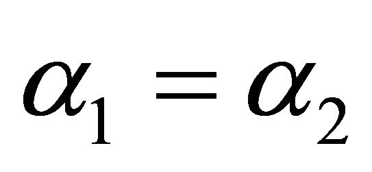Theorem. Let two-parameter LD and two-parameter LD. If and (or if and), then and hence, and.

Proof. We have

Now

.

Thus

(5.2)

Case (i) If and, then

.

This means that and hence

and.

Case (ii) If and, then

.

This means that and hence

and.

This theorem shows the flexibility of two-parameter LD over one parameter LD and exponential distributions.

6. Estimation of Parameters

6.1. Maximum Likelihood Estimates

Let be a random sample of size n from a two-parameter LD (2.1) and let be the observed frequency in the sample corresponding to

such that

where is the largest observed value having non-zero frequency. The likelihood function, of the two-parameter LD (2.1) is given by

(6.1.1)

and so the log likelihood function is obtained as

(6.1.2)

The two log likelihood equations are thus obtained as

(6.1.3)

(6.1.4)

Equation (6.1.3) gives, which is the mean of the two-parameter LD. The two Equations (6.1.3) and (6.1.4) do not seem to be solved directly. However, the Fisher’s scoring method can be applied to solve these equations. For, we have

(6.1.5)

(6.1.6)

(6.1.7)

The following equations for and can be solved

(6.1.8)

where and are the initial values of and respectively. These equations are solved iteratively till sufficiently close estimates of and are obtained.

6.2. Estimates from Moments

Using the first two moments about origin of the twoparameter Lindley distribution, we have

(6.2.1)

Taking, we get

.

This gives

(6.2.2)

which is a quadratic equation in. Replacing the first and the second moments and by the respective sample moments 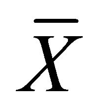and an estimate of can be obtained, using which, the Equation (6.2.2) can be solved and an estimate of obtained. Again, substituting in the expression for the mean of the two-parameter LD, we get

and thus an estimate of is given by

(6.2.3)

Finally, an estimate of is obtained as

(6.2.4)

7. Goodness of Fit

The two-parameter LD has been fitted to a number of data-sets relating to waiting and survival times to which earlier the one parameter LD has been fitted by others and to almost all these data-sets the two-parameter LD provides closer fits than the one parameter LD.

The fittings of the two-parameter LD to three such data-sets have been presented in the following tables. The data sets given in Tables 1-3 are the data sets reported by M. E. Ghitany, B. Atieh, and H. Nadarajah [3], T. Bzerkedal [9], and S. Paranjpe and M. B. Rajarshi [10] respectively. The expected frequencies according to the one parameter LD have also been given for ready comparison with those obtained by the two-parameter LD. The estimates of the parameters have been obtained by the method of moments.

Table 1. Waiting times (in minutes) of 100 bank customers.

Table 2. Data of survival times (in days) of 72 guinea pigs infected with virulent tubercle bacilli.

Table 3. Mortality grouped data for blackbird species.

It can be seen that the two-parameter LD gives much closer fits than the one parameter LD and thus provides a better alternative to the one-parameter LD for modeling waiting and survival times data.

8. Conclusion

In this paper, we propose a two-parameter Lindley distribution (LD), of which the one-parameter LD is a particular case, for modeling waiting and survival times data. Several properties of the two-parameter LD such as moments, failure rate function, mean residual life function, stochastic orderings, estimation of parameters by the method of maximum likelihood and the method of moments have been discussed. Finally, the proposed distribution has been fitted to a number of data sets relating to waiting and survival times to test its goodness of fit to which earlier the one-parameter LD has been fitted and it is found that two-parameter LD provides better fits than those by the one-parameter LD.

9. Acknowledgements

The authors express their gratitude to the referees for valuable comments and suggestions which improved the quality of the paper.

REFERENCES

- D. V. Lindley, “Fiducial Distributions and Bayes’ Theorem,” Journal of the Royal Statistical Society, Series B, Vol. 20, No. 1, 1958, pp. 102-107.
- D. V. Lindley, “Introduction to Probability and Statistics from Bayesian Viewpoint,” Cambridge University Press, New York, 1965. doi:10.1017/CBO9780511662973
- M. E. Ghitany, B. Atieh and S. Nadarajah, “Lindley Distribution and Its Applications,” Mathematics and Computers in Simulation, Vol.78, No. 4, 2008, pp. 493-506. doi:10.1016/j.matcom.2007.06.007
- E. G. Deniz and E. C. Ojeda, “The Discrete Lindley Distribution-Properties and Applications,” Journal of Statistical Computation and Simulation, Vol. 81, No. 11, 2011, pp. 1405-1416. doi:10.1080/00949655.2010.487825
- M. Sankaran, “The Discrete Poisson-Lindley distribution,” Biometrics, Vol. 26, No. 1, 1970. pp. 145-149. doi:10.2307/2529053
- J. Mazucheli and J. A. Achcar, “The Lindley Distribution Applied to Competing Risks Lifetime Data,” Computer Methods and Programs in Biomedicine, Vol. 104, No. 2, 2011, pp. 188-192. doi:10.1016/j.cmpb.2011.03.006
- M. E. Ghitany, F. Alqallaf, D. K. Al-Mutairi and H. A. Hussain, “A Two Parameter Weighted Lindley Distribution and Its Applications to Survival Data,” Mathematics and Computers in Simulation, Vol. 81, No. 6, 2011, pp. 1190-1201. doi:10.1016/j.matcom.2010.11.005
- H. S. Bakouch, B. M. Al-Zahrani, A. A. Al-Shomrani, V. A. A. Marchi and F. Louzada, “An Extended Lindley Distribution,” Journal of the Korean Statistical Society, Vol. 41, No. 1, 2012, pp. 75-85. doi:10.1016/j.jkss.2011.06.002
- T. Bjerkedal, “Acquisition of Resistance in Guinea Pigs Infected with Different Doses of Virulent Tubercle Bacilli,” American Journal of Epidemiology, Vol. 72, No. 1, 1960, pp. 130-148.
- S. Paranjpe and M. B. Rajarshi, “Modeling Non-Monotonic Survivorship Data with Bath Tube Distributions,” Ecology, Vol. 67, No. 6, 1986, pp. 1693-1695. doi:10.2307/1939102