Int'l J. of Communications, Network and System Sciences
Vol.3 No.1(2010), Article ID:1182,9 pages DOI:10.4236/ijcns.2010.31015
Extending the Network Lifetime of Wireless Sensor Networks Using Residual Energy Extraction—Hybrid Scheduling Algorithm
1Department of ECE, Anna University, Tamil Nadu, India
2Department of Information Technology, Sona College of Technology, Tamil Nadu, India
E-mail: tvpssn@gmail.com, chitra_slm@yahoo.com
Received July 2, 2009; revised September 29, 2009; accepted November 3, 2009
Keywords: Wireless Sensor Networks, Lifetime, Residual Energy, Hybrid Algorithm
Abstract
Wireless sensor networks (WSNs) are mostly deployed in a remote working environment, since sensor nodes are small in size, cost-efficient, low-power devices, and have limited battery power supply. Because of limited power source, energy consumption has been considered as the most critical factor when designing sensor network protocols. The network lifetime mainly depends on the battery lifetime of the node. The main concern is to increase the lifetime with respect to energy constraints. One way of doing this is by turning off redun-dant nodes to sleep mode to conserve energy while active nodes can provide essential k-coverage, which improves fault-tolerance. Hence, we use scheduling algorithms that turn off redundant nodes after providing the required coverage level k. The scheduling algorithms can be implemented in centralized or localized schemes, which have their own advantages and disadvantages. To exploit the advantages of both schemes, we employ both schemes on the network according to a threshold value. This threshold value is estimated on the performance of WSN based on network lifetime comparison using centralized and localized algorithms. To extend the network lifetime and to extract the useful energy from the network further, we go for compromise in the area covered by nodes.
1. Introduction
In recent years, wireless sensor network (WsSN) has been mainly used in applications such as health, military, and environmental monitoring. This growth has been fueled by its widespread popularity in wireless communication. However, there are limitations due to energy constraints. Because of the energy level variation, the network lifetime gets reduced. Therefore, considerable effort is needed to make it more efficient. To maximize the network lifetime, the energy consumption of the node should be reduced. Recently, a major research in this area has been on the use of centralized and localized k-coverage algorithms. The proposed algorithm states that depending on the network size, the network is reconfigured to any one of the algorithms to minimize the energy wastage.
2. Related Works
Various approaches for reducing the energy expenditure have been presented in literature; several papers minimize the transmitter power (a significant energy drain for WSN nodes) while maintaining connectivity by aggregation techniques [1,2], by using mobility of sinks [3,4]. Several routing protocols [5,6] showed significant improvements in the network lifetime for ad hoc networks (MANETs) and WSN by choosing routes that avoid nodes with low battery and by balancing the traffic load. Approaches at the medium access control (MAC) layer are geared towards reducing idle listening power and decreasing the number of collisions [7,8]. Applicationlayer approaches show dramatic energy savings for several classes of applications. The works in [9] deal with the target coverage problem where the purpose is to cover all the targets. The authors proposed an LP-based algorithm, which extends network lifetime by organizing the sensors to subsets, which are activated successively and only the active sensors are responsible for monitoring the targets. The works in [10,11] deal with area coverage problem where the main objective is to cover an area. Approaches to this problem are to divide sensors into disjoint or non-disjoint sets, such that each set can monitor every point in the surveillance area and all sets are activated successively so as to increase network lifetime.
In this paper, we focus on scheduling decisions that maximize the lifetime of the WSN. If the network is dead (due to some nodes) with respect to 100% coverage area, then we can reduce the percentage area coverage to 80% and then start monitoring. This process can be repeated by reducing coverage levels.
3. Algorithms
The algorithms used here assume a two-dimensional area with randomly deployed set of sensors S ={s1, s2, ..., sn} with a fixed sensing range r. In this paper, we have three main parts to solve. The first part deals with finding out the coverage of each sensor. The second part deals with the disjoint set formation/node scheduling algorithm development. The third part deals with the employment of the centralized algorithm in a given topology with different percentages of area covered.
3.1. Algorithm to Find k-Coverage
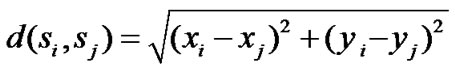
We are given a set of sensors, S ={s1, s2, ..., sn}, in a two-dimensional area A. Each sensor sensor si, i = 1, ..., n, is located at coordinate (xi, yi )inside A and has a sensing range of ri, i.e., it can monitor any object that is within a distance of ri from si .A location in A is said to be covered by si if it is within si’s sensing range. A location in A is said to be j-covered if it is within at least j sensors’ sensing ranges. Here, we use an algorithm to determine whether a sensor is k-perimeter-covered or not. Consider two sensors si and sj located in positions (xi, yi) and (xj, yj ), respectively. The distance between the two sensors is calculated using the distance Equation (1) d (si, sj)
 (1)
(1)
If d(si, sj)> 2r, then sj does not contribute any coverage to si’s area coverage. The fraction of coverage is given by finding the segment of si overlapping with sj using the central angle. The central angle can be noted from Figure 1, which can be derived by considering the Δpsisj. Using the cosine rule, the central angle can be found, which can be obtained from (2)
 (2)
(2)

Figure 1. Central angle.
 (3)
(3)
This can be repeated for all sensors that overlap with si as follows.
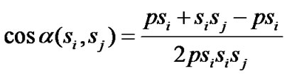
1) For all neighboring sensors sj of si such that d(si, sj)>2r, place the points αj,L and αj,L R on the line segment [0,2π] and sort all these points in an ascending order into a list L. Properly mark each point as a left or right boundary of a coverage range.
2) Traverse the line segment [0,2π] by visiting each element in the sorted list L from left to right. If αj,L comes, add the coverage by 1, whereas if αj,R comes, decrement the coverage by 1 to determine the coverage of si.
3.2. Scheduling Algorithm
Energy is a restricted resource for sensors, which determines how long and how well sensor networks can work. To save energy, most energy-efficient approaches reduce the number of sensors working simultaneously. By scheduling redundant sensors to go to sleep while the essential coverage has been satisfied, the network lifetime can be significantly extended.
3.2.1. Centralized Scheduling Algorithm
The network lifetime is defined as the total duration during which the whole area is k-covered. Sensor scheduling for k-coverage (SSC) can be defined as a sensor network with n sensors that can provide k-coverage for the monitored area, schedule the activities of the sensors such that at any time, the whole area can be k-covered and the network lifetime is maximized.
The scheduling decisions can be made at the Base Station (BS). The BS broadcasts the schedule to all the sensors so that each sensor can know when it should be active to monitor the area. Hence, the name centralized scheduling for k-coverage algorithm (CSKA). To solve the SSC problem, we can divide the sensors into disjoint or non-disjoint subsets and each subset k-covers the whole area, where k-cover implies that for every point in the area, it is covered (monitored) by at least k sensors. These subsets can be scheduled to be active successively. For each subset, its lifetime is determined by the sensor that has the least power.
Consider sensor si is k-perimeter covered if all points on the perimeter of si are covered by at least k sensors, which are in the same set with si, other than si itself. Similarly, a segment of si’s perimeter is k-perimetercovered if all the points on the segment are covered by at least k sensors, which are in the same set with si, other than si itself. The perimeter coverage level (PCL) of a sensor si is defined as the number of sensors in the same set with si, which cover any point on si’s perimeter of the sensing area. The lower the PCL, the smaller will be the node density.
Considering the case where each sensor has a fixed sensing range and all the sensors are divided into disjoint cover sets, our goal is to construct as many subsets as possible such that 1) each subset can k-cover the whole monitored area; 2) the network lifetime is maximized.
Figure 2 shows the explanation of PCLGreedySelection algorithm, which is used to form disjoint subsets. The input of this algorithm is the required coverage level k, the sensor set {S}. The main idea is to iteratively construct subsets Ci by choosing sensors from the region with the lowest sensor density. When constructing an individual Ci, at each step, the sensor with the smallest PCL value is added to Ci. In this way, we can include as few sensors as possible in Ci and these sensors are distributed in the area as widely as possible because they are from the regions with the lowest sensor density, such that more sensors can be left to join other subsequent subsets and the overlapped sensing regions in each subset are reduced as much as possible. This also indicates that when constructing a subset Ci, the region with

Figure 2. PCLGreedySelection algorithm.
 (a)
(a) (b)
(b)
Figure 3. Perimeter coverage of a sensor si.
smaller node density is taken care of with higher priority. The output of this algorithm is the number of disjoint subsets {C}, which provide essential k-coverage.
The input of this algorithm includes k, the user-specified coverage level, and S, the set of all the sensors. The output is Ci, a set of subsets, and each subset can k-cover the whole area. To verify whether a subset Ci can k-cover the entire surveillance area, the method used is proposed in [10] and is called get Coverage Level (Ci).
Figure 3 shows the perimeter coverage of sensor si. For each sensor si, it tries to identify all neighboring sensors that can contribute some coverage to si’s perimeter. Specifically, for each neighboring sensor sj, we can determine the angle of si’s arch, denoted by [αj, L, αj, R], which is perimeter-covered by sj. Placing all angles [αj, L, αj, R] on [0,2π] for all j’s, it is easy to determine the level of perimeter coverage of si. For example, Figure 3(a) shows how si is covered by its neighbor nodes (shown in dashed circles). Figure 3(b) shows that mapping these covered angles decide that si is perimeter covered. After coverage verification, all the sensors in S are sorted in non-decreasing order based on their PCL values. Then, sensors are added into a subset in a greedy manner. If at some iteration, the current subset Ci can provide k-coverage, a new subset Ci 1 will be constructed in the same manner. PCLGreedySelection stops when we can no longer construct subsets that can k-cover the whole surveillance area.
The subsets formed using PCL algorithm will have redundant sensors, since each node is added to subset in a greedy manner. These redundant sensors are identified and removed and added back to S so that they are still available to be added to the subsequent subsets. This operation is performed using the subroutine called Prune GreedySelection algorithm, which is shown in Figure 4. In this algorithm, given a subset Ci, each sensor in Ci is checked to see whether sensor coverage scovi is smaller than the user-specified k value by removing each and every sensor in that subset.
If a sensor is redundant (after removing this sensor from Ci, scovi is still not smaller than k), it will be removed from Ci and added back to S so that it can be used to form other subsets.
The PCLGreedySelection algorithm and PruneGreedySelection algorithm together constitute the centralized scheduling algorithm (CSA). CSA is first employed to form disjoint subsets such that every subset covers 95% of the surveillance area. When the network fails, some/ most of the nodes may have enough energy to work more.
3.2.2. Localized Scheduling for k Coverage Algorithm (LSKA)
LSKA works in a rounding fashion as in Figure 5 with
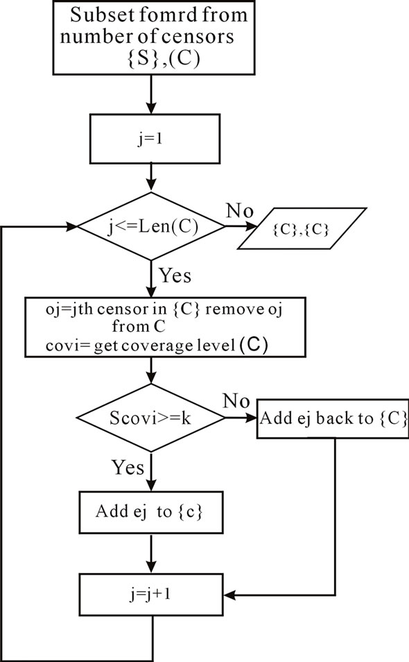
Figure 4. PruneGreedySelection algorithm (k, S, Ci).
the round length of dRound, meaning that each sensor runs this algorithm every dRound unit of time. At the beginning of each round is a decision phase with the duration of W. There are several advantages of working in rounds.
1) k can be dynamically changed. For some applications, such as forest fire, the value of k needs to be changed while the network is running. For example, in the dried season, there is more chance of fire happening, thus the value of k needs to be high. However, in the rainy season, that chance is small, so the value of k needs to be small to save network energy. Also, the operation of the network does not need to be interrupted while k is being changed.
2) LSKA supports robustness. At each round, there is exactly one set cover responsible for sensing task. In a situation that some sensors in that set cover are out of service (may die, for example), the sensing data will be affected and network may temporarily not provide k-coverage for some interval of time. However, this problem will not affect for long, since the new set cover will be discovered at the next round to take charge of the sensing task.
3) Energy-efficient algorithm. LSKA is an energyefficient distributed algorithm, which requires only 1-sensing hop neighbor information and it also provides kcoverage for the whole network (which is a kind of faulttolerance). Thus, LSK algorithm satisfies all the requirements of a sensor network protocol.
All the sensors have to decide their status in the decision phase. The decision time “W” here is the time taken to compute the status once. The status of the sensors can be ON or OFF and each sensor decides its status sequentially and informs the status through the “HELLO” messages to its neighbors. Each neighbor finds its neighbors and updates the value using the already received “HELLO” messages.
And in the sensing phase, the sensor that decided to remain ON begins to monitor the area and sends the updated data messages. The “HELLO” messages consume a considerable amount of energy. Hence, to eliminate this, it is assumed that dRound >>W. Here, dRound is assumed to be 15 times “W”.
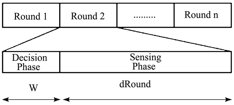
Figure 5. Localized scheduling rounds.
4. Energy Model and Simulation Setup
The radio energy model that is being used in our analysis is shown in Figure 6. A simple model is assumed where the transmitter dissipates energy to run the radio electronics and the power amplifier and the receiver dissipates energy to run the radio electronics.
For our simulation, a variable-size network both of grid and random topologies are used where nodes were distributed between (x=0, y=0) and (x=100, y=100) with the Base Station at location x=10, y=50. Each data message is 2 Kbits long and hello messages are 200 bits long. The power attenuation is dependent on the distance between the transmitter and the receiver. For relatively short distances, the propagation loss can be modeled as inversely proportional to d2, whereas for longer distances, the propagation loss can be modeled as inversely proportional to d4.
In this simulation, the free space (power loss) channel models were used. The electronic energy Eelec is the energy consumed in the electronics circuit to transmit or receive the signal, which depends on factors such as digital coding, modulation, and filtering of the signal before it is sent to the transmit amplifier. The amplifier energy Eamp* d2 depends on the distance to the receiver and the acceptable bit-error rate. It is assumed that this d2 energy loss is due to channel transmission. For the simulation described in this paper, the communication energy parameters are set as: Eelec =50 nJ/bit, Eamp =10 pJ/bit/ m2. A simple radio model has been used as in [11,12]
Transmitter:
 ; if d< dc
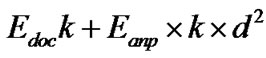 ; Otherwise (4)
Receiver: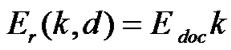 (5)
(5)
where dc is the cross-over distance, k is the packet bit size, and d is the distance between transmitter and receiver antennas.
5. Simulation Results
The proposed work involves the employment of CSKA and LSKA in the networks of various sizes using the above-described energy model. The research works currently going on employ either CSKA or LSKA alone, but both algorithms have their own advantages and disadvantages.
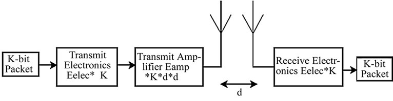
Figure 6. Radio model.
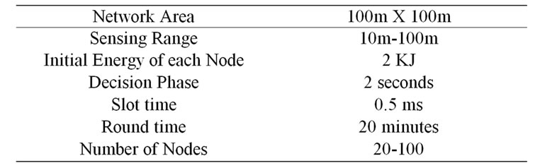
Table 1. Simulation setup.
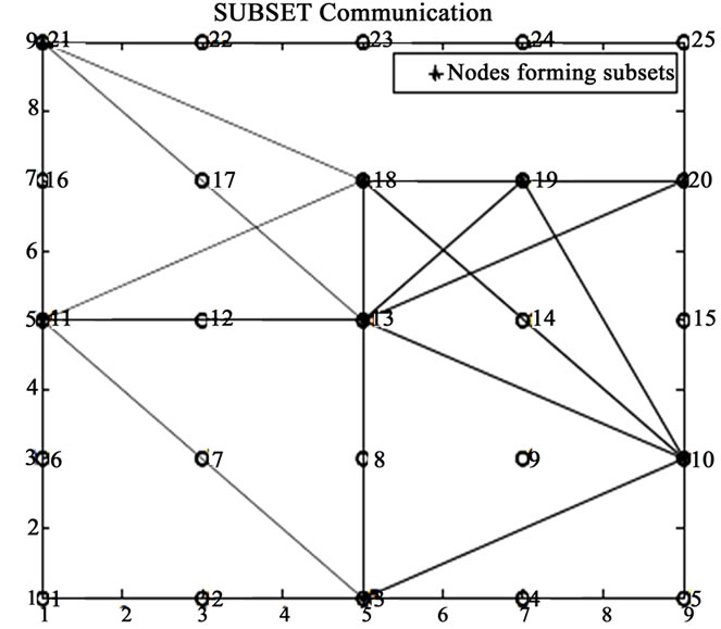
Figure 7. Sample of random deployment.
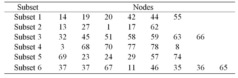
Table 2. Disjoint subsets.
Hence, to exploit the advantages of both algorithms, we use CSKA and LSKA in the same network. For this, a threshold should be found for when to switch from one algorithm to next to maximize the network lifetime. Table 1 shows the simulation setup.
5.1. Deployment and Subset Formation
Figure 7 shows the sample for a random deployment of 100 nodes in the two-dimensional area of 100 ´ 100 m2, which monitors the entire coverage region with redundant nodes. These redundant nodes can be used to form subsets such that every subset can cover the entire surveillance area. The assumptions are made such that each sensor has the sensing range of 3 m and communication range as twice the sensing range to ensure connectivity. By using PCL and PruneGreedy algorithm, six disjoint subsets are formed from the 100 deployed nodes. Table 2 shows the disjoint subsets. From the subsets formed, it is found that each sensor participates in only one subset, hence the name disjoint subsets.
5.2. Number of Nodes and Subsets
From Figure 8, it is found that the number of subsets increases as the number of nodes increases. Also, when the number of nodes is 300, 12 disjoint subsets are formed when K=1 and only 2 disjoint subsets are formed when K=2. From the graph, we know that as k increases, the number of subsets decreases, since more sensors are needed per subset to achieve the required coverage.
5.3. Network Lifetime Comparison with CSK Algorithm
Figure 9 infers that the network lifetime is increased by using the CSKA algorithm. The network lifetime is given in terms of rounds until all the subsets die. A subset is assumed to be useless when one of the sensor’s energy is below the threshold. Also, it shows that if the coverage level increases from k=1 to k=2, the network lifetime decreases. This is because the number of nodes in the

Figure 8. Number of nodes vs. subsets.

Figure 9. Deployed sensors vs. network lifetime (CSKA).
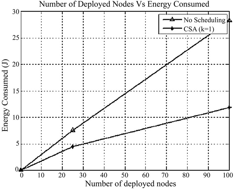
Figure 10. Deployed sensor nodes vs. energy consumption.
subset increases if the required coverage level k increases. The results show that without scheduling, the lifetime of the network when the 100 nodes are deployed in the surveillance area is only 0.2 ´ 104 time slot, whereas with the scheduling algorithm when coverage level k =2, the network lifetime is 4 ´ 104 time slot. By using scheduling algorithm, the lifetime of the network is improved 20 times than that without the scheduling scheme.
5.4. Energy Consumption
Figure 10 shows that CSKA algorithm reduces energy consumption because of the less number of redundant neighbors and hence redundant message transmissions. By using scheduling algorithm, 53% energy is saved when compared to the case without scheduling scheme.
5.5. Sensing Range and Subsets
Figure 11 illustrates that as the sensing range increases, the number of subsets formed increases. This happens because only less number of sensors is needed to provide the same coverage. That is, with larger sensing ranges, the number of sensors in each subset decreases such that more subsets can be constructed. When the sensing range is 50 m and the number of nodes is 100, then the number of disjoint subsets is 8, and when the sensing range is 100 m, the number of disjoint subsets is 18 because of less number of sensors in each subset.
5.6. Sensing Range and Number of Sensors per Subset
Figure 12 shows that as the sensing range increases, the number of sensors covered by each subset get reduced because only less number of sensors is needed to provide the same coverage. When the number of sensors deployed in the application area is 100 and sensing range is 50 m,
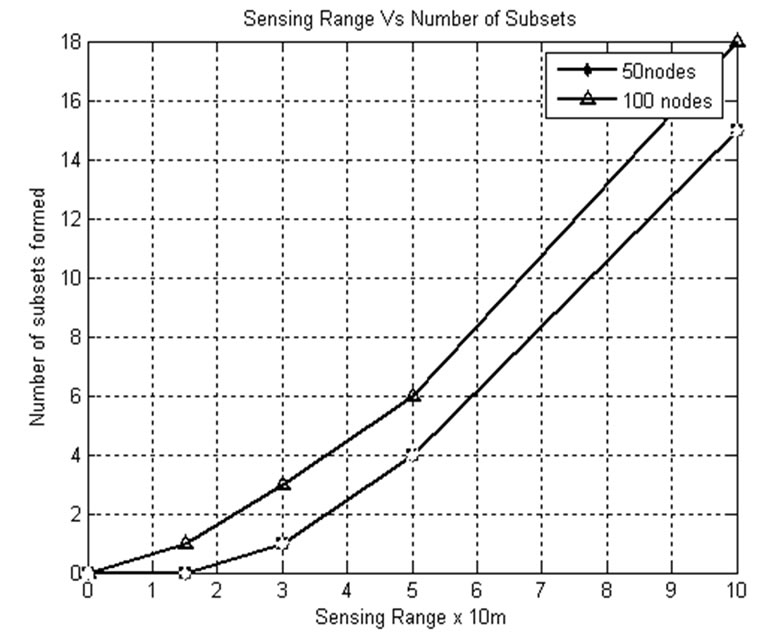
Figure 11. Sensing range vs. number of subsets.
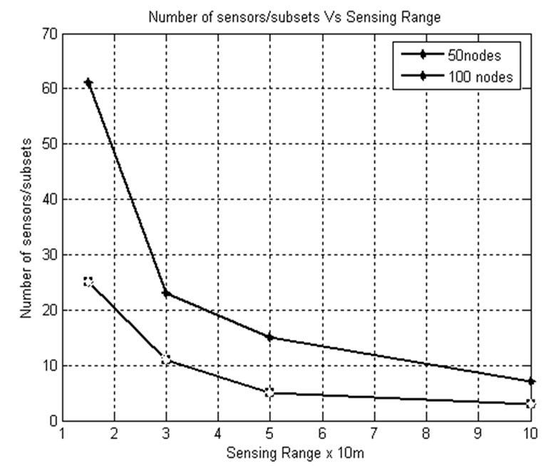
Figure 12. Sensing range vs. number of sensors/subsets.
only 10 sensors are covered by each subset, whereas when the sensing range is 100 m for the same number of sensors deployed in the application area, 3 sensors are covered by each subset. From this, we know that as the sensing range increases, the number of subsets formed get increased.
5.7. Residual Energy Extraction and Node Utilization by Varying Area Coverage Levels
Using disjoint subset algorithms, only 30% of the deployed sensors are utilized in subset formation; the remaining nodes are not used. Hence, to utilize those nodes, here it is opted to go for the compromise in area. Thus, by compromising in area, more number of nodes is utilized, residual energy is reduced, and network lifetime is improved.
5.7.1. Number of Utilized Sensors
From Figure 13, it is observed that when centralized scheduling algorithm is applied, the number of utilized nodes are much less than the available nodes, and hence to use all or most of the deployed sensors, as a part of the work, an idea to go for compromise in area coverage is developed here. The usage of most of the deployed sensors and reduced residual energy is ensured from the work.
5.7.2. Lifetime Comparison with Varying Area Coverage Levels
The CSKA first uses the subsets formed by 95% of the whole monitored area. When all the subsets are dead, the percentage of coverage level is changed from 95 to 85%. This ensures the usage of the nodes that are not used in the earlier rounds. This process is repeated till we get the acceptable level of coverage that can be used. Here, it is assumed that the monitoring service requires at least 50% of coverage. Figure 14 shows the improvement in network lifetime by employing the CSKA to variable area coverage levels. If 95% of area alone is considered,

Figure 13. Number of utilized sensors.
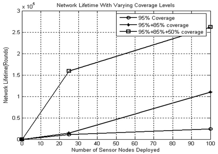
Figure 14. Lifetime comparison with varying area coverage levels.
only less number of nodes is used in subset formation and in monitoring service. Even though there are some nodes available with enough energy, the network is announced dead. To avoid this, residual energy is extracted from the nodes that are still alive.
5.7.3. Residual Energy Utilization
Figure 15 confirms that the remaining (residual) energy from the network is extracted and utilized in the monitoring service. The nodes that are not used are also involved in subset formation of the subsequent rounds so that utilization of the nodes is also increased.
5.7.4. Node Utilization
From Figure 16, it is observed that the number of nodes that are not used is decreased by the usage of CSKA algorithm by varying the area to be covered. In other words, it can be said that the utilization of nodes is increased by the compromise in area coverage level from 95 to 80% and so on.

Figure 15. Residual energy utilization.
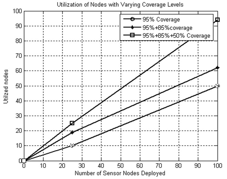
Figure 16. Node utilization.

Figure 17. Network lifetime comparison for k=1.
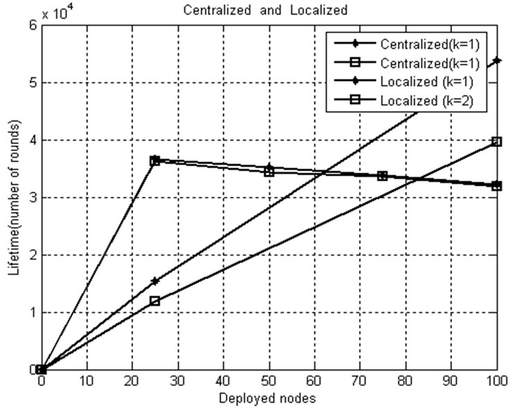
Figure 18. Network lifetime comparison for k=1, k=2.
5.7.5. Network Lifetime Comparison for k=1
As explained earlier, the aim of the thesis is to find the threshold to switch from CSKA to LSKA and vice versa to improve the network lifetime of the WSN. This can be done by employing CSKA and LSKA on the networks of various sizes deployed in the same area. Figure 17 shows the network lifetime comparison for k=1 with and without applying scheduling algorithms. The lifetime in localized scheme is lesser when compared to that of the centralized scheme because of the frequent exchange of hello packets. The graph illustrates that for the given conditions, the localized scheduling algorithm provides better results when the network size is less than 60 nodes and above that the centralized scheduling algorithm takes over.
5.7.6. Network Lifetime Comparison for k=1, k=2
Figure 18 shows the relationship between network lifetimes, desired coverage level k, network size threshold value to switch from centralized to localized algorithm and vice versa. From the figure, it can be seen that when k increases, the network lifetime decreases. Also, it comes into light that as k increases, the network size threshold increases, since a greater number of nodes are used to cover the monitored area with increased coverage level (k=2). For k=1, the threshold is found as 61 nodes, whereas for k=2, it increases to 83 nodes. Thus, the threshold is proportional to the network size.
5.8. Conclusions and Future Work
In this paper, we used coverage-preserving centralized node-scheduling scheme to reduce energy consumption and therefore increase system lifetime, by turning off some redundant nodes. Further, to increase the network lifetime and to extract the residual energy from the remaining nodes, we change the monitoring area levels. The improvements obtained from the proposed scheme are an increase in the network lifetime by 30000–50000 rounds and a reduction in energy consumption by 41.2% to 58.09%, when compared to that without the scheduling scheme. However, it also infers that only about 30% of the deployed sensors are utilized in subset formation and the remaining nodes are not used. Hence, to utilize those nodes, here it is opted to go for the compromise in area. Thus, from the results, it is concluded that by compromising in area, more number of nodes are utilized, residual energy is reduced, and network lifetime is improved. From the results, we conclude that the localized algorithm provides better performance than the centralized one when the network size is smaller. That is when the network has 25 nodes, it provides 21,000 rounds greater life. But when the network size increases, the exchange of hello packets consumes a considerable amount of energy in LSKA. Hence, CSKA provides better results for larger networks. When the results of CSKA and LSKA are plotted in the same graph, a crossing point is found. This is the threshold to switch from LSKA to CSKA. This threshold to switch from one algorithm to another depends on the required coverage level k, the buffers required for nodes to store adjacent nodes information for localized algorithm, the sensing range, etc.
The future vision is to use the algorithm for the sensors with adjustable sensing range and to consider the buffer variation in network area to find the threshold expression.
6. References
[1] S. Zou, J. I. Nikolaidis, and J. J. Hames, “Extending sensor network lifetime via through first hop aggregation,” IEEE Mobile Computing, 2006.
[2] W. Yu, T. Nam Le, D. Xuan, and W. Zhao, “Query aggregation for providing efficient data services in sensor networks,” Proceedings of IEEE International Conference on Mobile Ad Hoc and Sensor Networks, 2004.
[3] Z. M. Wang, S. Basagni, E. Melachrinoudis, and C. Petrioli, “Exploiting sink mobility for maximizing sensor networks lifetime,” Proceedings of the 38th Hawaii International Conference on System Sciences, 2005.
[4] S. Basagni, A. Carosi, and M. Wang, “Controlled sink mobility for prolonging wireless sensor network lifetimes,” Springer Science + Business Media, LLC, 2007.
[5] J. Aslam, Q. Li, and D. Rus, “Three power-aware routing algorithms forsensor networks,” Wireless Communications and Mobile Computing, Vol. 2, No. 3, pp. 187–208, March 2003.
[6] W. Heinzelman, J. Kulic, and H. Balakrishnan, “Adaptive protocols for information dissemination in wireless sensor networks,” in Proceedings of ACM/IEEE MobiCom, pp. 174–185, August 1999.
[7] W. Ye, J. Heidemann, and D. Estrin, “An energy-efficient MAC protocol for wireless sensor networks,” in IEEE INFOCOM 2002, June 2002.
[8] T. V. Dam and K. Langendoen, “An adaptive energyefficient MAC protocol for wireless sensor networks,” in ACM Sensys’03, November 2003.
[9] M. Cardei and D. Z. Du, “Improving wireless sensor network lifetime through power aware organization,” Springer Science + Business Media, 2005.
[10] F. H. Chi, C. T. Yu, and L. W. Hsiao, “Distributed protocols for ensuring both coverage and connectivity of a wireless sensor network,” National Chiao-Tung University, Springer Science, 2003.
[11] W. Heinzelman, A. Chandrakasan, and H. Balakrishnan, “An application—Specific protocol architecture for wireless micro sensor networks,” IEEE Transactions on Wireless Communications, Vol. 1, No. 4, pp. 660–670, October 2002.
[12] W. Heinzelman, A Chandrakasan, and H. Balakrishnan, “Energy-efficient communication protocol for wireless micro sensor networks,” Proceedings of the 33d Annual Hawaii International Conference on System Sciences, pp. 3005–3014, 2000.