Journal of Environmental Protection
Vol. 3 No. 7 (2012) , Article ID: 21141 , 24 pages DOI:10.4236/jep.2012.37079
Temporal Trends in Ambient SO2 at a High Altitude Site in Semi-Arid Western India: Observations versus Chemical Transport Modeling
![]()
Physical Research Laboratory, Ahmedabad, India.
Email: timmyf@prl.res.in
Received March 18th, 2012; revised April 19th, 2012; accepted May 22nd, 2012
Keywords: SO2; GEOS-Chem; HYSPLIT; IOCL Oil Fire; PBL Height; OH Radical
ABSTRACT
Ambient sulphur dioxide (SO2) measurements have been performed at a high altitude site in the semi arid region of western India, Gurushikhar, Mt. Abu (24.6˚N, 72.7˚E, 1680 m ASL), during different sampling periods span over Sep-Dec 2009 and Feb-Mar 2010. A global three dimensional chemical transport Model, GEOS-Chem, (v8-03-01) is employed to generate the SO2 profile for the entire region for the different sampling months which in turn is used to explain the major features in the measured SO2 spectra via correlating with HYSPLIT generated wind back trajectories. The mean SO2 concentrations recorded at the sampling site varied for the different sampling periods (4.3 ppbv in Sep-Oct 2009, 3.4 ppbv in Nov 2009, 3.5 ppbv in Dec 2009, 7.7 ppbv in Feb 2010 and 9.2 ppbv in Mar 2010) which were found to be strongly influenced by long range transport from a source region surrounding 30˚N, 75˚E—the one projected with the highest SO2 concentration in the GEOS-Chem generated profiles for the region—lying only a few co-ordinates away. A diurnal cycle of SO2 concentration exists throughout the sampling periods, with the greatest day-night changes observed during Feb and Mar 2010, barely detectable during Sep-Oct 2009, and intermediate values for Nov and Dec 2009 which are systematically studied using the time series PBL height and OH radical values from the GEOS-Chem model. During the sampling period in Nov 2009, a plume transport to the sampling site also was detected when a major fire erupted at an oil depot in Jaipur (26.92˚N, 75.82˚E), located few co-ordinates away. Separate runs of the model, performed to study the long range transport effects, show a drop in the SO2 levels over the sampling region in the absence of transport, throughout the year with Jan to Apr seen to be influenced the lowest by long range transport while Jul and Dec influenced the highest.
1. Introduction
The present day increased fossil fuel and coal usage in Asia, to meet the energy needs of a rapidly emerging economy, has raised concerns about the potential threats of sulphur dioxide (SO2) emission from this region [1-5] to the global climate. Further, there exist many recent reports [6-8]—based on direct observations as well as chemical transport modeling studies—of SO2 from Asia out-flowing to the western Pacific and influencing the climatology of this region.
In urban areas it is the fossil fuel combustion which contributes to the majority of the anthropogenically produced SO2, releasing over 90% of the sulphur content in these fuels to the atmosphere as sulphur dioxide [9,10]. With the known prominent roles of SO2 in the chemistry of the global troposphere [11-18] and in the sulphur cycle including its potential to interfere with the oxidizing power of the atmosphere, to cause acid rain (e.g., [19, 20]), and to modify the atmospheric radiative forcing pattern via gas-phase chemistry and particle formation, there is an impending need to monitor systematically the emission and transport pattern SO2 over different region in Asia, with differing environmental conditions.
As a special case, the monitoring of ambient SO2 levels coupled with wind trajectory analysis at a location devoid of local emissions and situated at free tropospheric altitudes (seasonal entry into the free troposphere when the planetary boundary layer (PBL) height is low) can help improve the present understanding of the free tropospheric transport patterns of SO2 from source to remote locations. Keeping this as one of the major goals, ambient SO2 concentrations were measured at a high altitude site in the semi arid region of western India, Gurushikhar, Mt. Abu (24.6˚N 72.7˚E, 1680 m Above Sea Level (ASL)), during Sep-Oct’09, Nov’09, Dec’09, Feb’10 and Mar’10. In this study a global three dimensional chemical transport model, GEOS-Chem, (v8-03- 01) is also employed, to generate the SO2 profiles for the entire region for the different sampling months to identify the major SO2 source regions.
2. Materials and Methods
2.1. Site Description: Gurushikhar, Mount Abu (24.6˚N, 72.7˚E, 1680 m ASL)
The sampling site for this study, Gurushikhar, Mt. Abu (24.6˚N, 72.7˚E, 1680 m ASL) is a high altitude site in the semi-arid region of western India, having a more or less clean atmosphere with minimal local emissions. Gurushikhar is the highest mountain peak in the southern end of Aravali range of mountains in western India with an annual average rainfall of about 600 - 700 mm precipitating only during SW-monsoon. The Gurushikhar site, because of its high elevation, can enter the free tropospheric zone during the winter and post-monsoon months when the Planetary Boundary Layer (PBL) height is low over the region for low incoming solar radiation (insolation) rates, while during summer it gets accommodated within the PBL. This special characteristic makes the Mt. Abu site suitable for the kind of study mentioned above viz., assessing the free tropospheric transport pattern of SO2 from source to remote locations.
2.2. Experimental Setup
A primary UV fluorescence SO2 Monitor (Thermo—43i Trace Level Enhanced (TLE)) was employed for the monitoring of ambient SO2 levels during the different sampling periods. The performances of similar systems are reported elsewhere [21-23]. Calibrations were performed routinely with a standard SO2 gas (2 ppmv with N2 balance gas, Spectra, USA) and zero air using a dynamic gas calibrator (Thermo—146i). The integration time for the SO2 analyser was set at five minutes and the data was periodically downloaded to a computer for analysis.
2.3. The GEOS-Chem Model
The GEOS-Chem global 3-D chemical transport model (v8-03-01; http://acmg.seas.harvard.edu/geos/) employed for this study uses GEOS-5 assimilated meteorological observations—including winds, convective mass fluxes, mixed layer depths, temperature, clouds, precipitation, and surface properties—from NASA Global Modeling and Assimilation Office (GMAO). The GEOS-5 data have a temporal resolution of 6-h (3-hour resolution for surface fields and mixing depths) and horizontal resolution of 0.5˚ latitude × 0.667˚ longitude, with 72 levels in the vertical extending from surface to approximately 0.01 hPa. The GEOS-Chem model (v8-03-01) simulates the Ozone-NOx-VOC-aerosol chemistry [24,25] and elaborative simulation evaluations are provided in [25-28].
In the present work, simulations were carried out for Jan 2009-Apr 2010 at 4˚ × 5˚ resolutions with the runs initialized on 1st Jan 2009 using GEOS-Chem fields generated by a one year spin-up simulation at 4˚ × 5˚ resolution. The emission inventories EMEP [29], BRAVO [30], EDGAR [31], Streets inventory [32], CAC (http://www.ec.gc.ca/pdb/cac/cac_home_e.cfm), and EPA/ NEI05 were included in the model runs by setting all of them to “True” in the standard input.geos file. Unless mentioned otherwise, the parameters set in the input.geos file for the model runs are identical to the ones in the standard input.geos file, distributed with the GEOSChem codes (v8-03-01), with the simulation start/end dates and the ND49 diagnostics—to generate the time series data—modified.
2.4. GAMAP Visualization Toolkit
The GEOS-Chem Model outputs during different runs are plotted using the Global Atmospheric Model Analysis Package (GAMAP) (Version 2.15; http://acmg.seas.harvard.edu/gamap/) which is a selfcontained, consistent, and user-friendly software package written in IDL (Interactive Data Language). The package can read outputs from chemical tracer models (CTM’s) and visualize it via line plots, 2D plots, 2D animations, or 3D iso-contour surface plots.
2.5. The HYSPLIT Trajectory Model
The wind back trajectory analysis for this work employs the HYSPLIT (HYbrid Single-Particle Lagrangian Integrated Trajectory) model, developed by NOAA ARL [33, 34] which uses a modelled vertical velocity scheme and can depict the vertical motion of the relevant air parcel. The 7-day back trajectories plotted for altitudes 50, 500 and 3000 m above the ground level (AGL) are used to identify the origin and the transect of the air parcels reaching the sampling site.
3. Results and Discussions
Ambient SO2 measurements were performed during Sep-Oct’09, Nov’09, Dec’09, Feb’10 and Mar’10. The GEOS-Chem chemical transport model (v8-03-01) is used to generate the SO2 profile for the entire region surrounding the sampling site for the different sampling months to identify the major source regions. Now by analysing the back trajectories generated using HYSPLIT for the sampling periods—performed at different altitudes to investigate the source and the transport pathways of the air parcel, prior to its arrival to the sampling site— and correlating them with the GEOS-Chem generated SO2 plots showing the source regions, the major features in the measured spectra are explained.
3.1. SO2 Plots for Different Sampling Months from GEOS-Chem
The GEOS-Chem model (v8-03-01) runs were performed for Sep 2009 to Apr 2010, with the inventories discussed previously, to find out the major SO2 source regions in the vicinity of the sampling site. The output averaged for the first half of each sampling month was then plotted using GAMAP and is shown in Figure 1. The plots showed a region surrounding 30˚N, 75˚E with the highest SO2 concentration in the vicinity. With the sampling site, Gurushikhar located only a few co-ordinates away, a long range transport to the sampling site from this high SO2 region (surrounding 30˚N, 75˚E) is feasible under favourable wind conditions, including free tropospheric transport, for the high elevation of the sampling site.
3.2. Time Series SO2 Profile from GEOS-Chem
The time series SO2 profiles for the nearest co—ordinates to the Mt. Abu site possible with the model (26˚N, 75˚E), for the ground level (0 - 0.3 km AGL), also was generated during the GEOS-Chem runs by turning ON the ND49 diagnostics in the input.geos file. This model generated SO2 time series were then plotted for the sampling periods to make comparison with the experimental results. The data is also used to study the diurnal variabilities and its dependence on different atmospheric parameters such as Planetary Boundary Layer (PBL) height and OH radical concentrations.
3.3. SO2 Measurements at Mt. Abu
The measured SO2 time series profiles had distinctly different features during different sampling periods span over Sep-Oct’09, Nov’09, Dec’09, Feb’10, and Mar’10, and were found to be dictated by the transport patterns and climatology prevailed in the respective months. The major features in the SO2 spectra for different sampling months and its correlation with various atmospheric parameters are discussed below. A comparison of the experimental SO2 time series data with GEOS-Chem model generated one’s also is made for the different sampling periods.
3.3.1. Major Features: September-October 2009
During Sep-Oct 2009, when the winds were mostly from the South-West direction (as shown in Figure 2), with the 7 day back trajectories originating mostly from Arabian sea where SO2 concentration is a minimum in the GEOS-Chem generated plots (Figure 1), the SO2 time series showed a near constant continuum with very few spikes (Figure 3). The mean SO2 concentration for this sampling period is 4.3 ppbv. The spikes in the spectrum seen on the 2nd and 3rd of Oct 2009 correlate very well with a change in wind trajectory pattern (Figure 2) when an air parcel from the high SO2 source region surrounding 30˚N, 75˚E reached the sampling site.
The SO2 profile had minimal diurnal variability (Figure 4) which is explained as due to the low PBL heights as well as high atmospheric OH radical concentration during these months over the sampling region (as will be discussed in section 3.4). The PBL height for this month over the sampling region is amongst the lowest of the year and the sampling site Gurushikhar is more or less within the free troposphere, nullifying the PBL height variation effects and hence the observed minimum diurnal variation for the SO2 levels. Also the high OH radical concentration due to a higher water vapour content and incoming solar radiation (insolation) rate—the two parameters necessary for the production of OH radical in the atmosphere via photo chemistry—possibly makes sure sufficient oxidation of SO2 even when the concentration is high to minimise the diurnal variation in the SO2 oxidation efficiency. The very negligible contribution from long range transport during this sampling period—as almost all the back trajectories originated in the Arabian sea where the SO2 concentration is a minimum in the GEOS-Chem generated plots, resulting in non dependence of the measured SO2 levels on possible diurnal variability of wind pattern—can be another possible reason for the minimal diurnal variation in the SO2 levels. The GEOS-Chem generated plots for the sampling period (shown in Figure 3) however showed some diurnal variation in SO2 levels which may be attributed to the difference in the altitudes of the sampling site and the co-ordinates used in the model calculations (due to the constraint that at 4˚ × 5˚ resolution, the nearest possible grid point available with the model was 26˚N, 75˚E, where the terrain height may be different).
3.3.2. Major Features: November 2009
During Nov 2009 when the wind back trajectories (Figure 5) extended mostly to North-East, the SO2 profile showed short duration spikes superimposed on the back ground values. The mean of the SO2 concentrations recorded (Figure 6) for this sampling period is 3.4 ppbv. For this month, the wind back trajectories showed occasional long range transport from the high SO2 region (surrounding 30˚N, 75˚E) along with those from the low SO2 regions (e.g., regions lying in the North-East of the sampling site) in the GEOS-Chem generated plots.


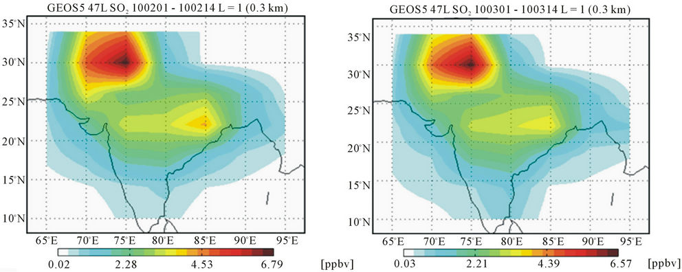
Figure 1. SO2 concentration (ppbv) over the region surrounding the sampling site, averaged for the first half of the different sampling months showing the major source regions, generated via GEOS-Chem model runs.
Because of the wind pattern specific for this month, only short duration random air parcels arrive at the sampling site at Mt. Abu from the high SO2 region surrounding 30˚N, 75˚E—as shown by the back trajectory analysis (Figure 5)—explaining the observed short duration spikes in the SO2 profile.


Figure 2. The wind back trajectories plotted for various days during the sampling period in Sep-Oct 2009 using HYSPLIT.

Figure 3. The SO2 time series recorded during the sampling period in Sep-Oct 2009 at Mt. Abu. The GEOS-Chem generated SO2 spectrum for the co-ordinates 26˚N, 75˚E—the nearest grid point available with the model at 4˚ × 5˚ resolution—also is shown for comparison.

Figure 4. The diurnal pattern for the SO2 concentration measured during the sampling period in Sep-Oct 2009 at Mt. Abu.
A diurnal pattern is observed (Figure 7) in the measured SO2 spectra, which may be attributed to the combined effects put in by the insolation dependent variation in OH radical levels and PBL height as well as the diurnal variation in the wind pattern carrying polluted air parcel to the sampling site from long distances.
The spikes as well as the concentration levels decreased from 12th Nov 2009, as is the case with the GEOS—Chem generated SO2 time series shown also in Figure 6—which has association with the wind trajectory change from high SO2 regions surrounding 30˚N, 75˚E to relatively low SO2 regions lying North-East of the sampling site.
Detection of SO2 Plume during a Major Oil Fire Incident A major fire had erupted at an oil depot of Indian Oil Corporation Limited (IOCL) at Jaipur, Rajasthan (26.92˚N, 75.82˚E) on 29th October 2009 at around 7:30 PM (IST). Approximately 60,000 kilolitres of oil were burned in this fire incident which lasted for almost a week till 6th Nov 2009, resulting in a significant rise in the air pollution levels over the region.
Studying the possible long range transport of SO2 containing plumes to the high altitude sampling site at Mt. Abu from the disaster site, located only a few co-ordinates away was another objective of the sampling for this month. Three short duration high intensity spikes were recorded (Figure 8) each on 2nd (around 0125 hrs) 4th


Figure 5. The wind back trajectories plotted for various days during the sampling period in November 2009 using HYSPLIT. The trajectories clearly showed the plume transport from the oil fire site (26.92˚N, 75.82˚E) during 2nd, 4th and 5th Nov 2009.

Figure 6. The SO2 time series recorded during the sampling period in November 2009 at Mt. Abu. The GEOS-Chem generated SO2 spectrum for the co-ordinates 26˚N, 75˚E also is shown for comparison.
(around 2230 hrs) and 5th (around 2120 hrs) of Nov 2009 which was found associated with this major oil fire from back trajectory analysis—which showed air parcels reaching the sampling site from the disaster site (26.92˚N, 75.82˚E), during the above days (Figure 5).
3.3.3. Major Features: December 2009
During Dec 2009, the winds—as seen in the back trajectory plots shown in Figure 9—were mostly from North and North-East of the sampling site and occasionally carried high SO2 from the source region surrounding

Figure 7. The diurnal pattern for the SO2 concentration measured during the sampling period in November 2009 at Mt. Abu.

Figure 8. The SO2 spikes detected at Mt. Abu when plumes from the Jaipur oil fire site (26.92˚N 75.82˚E) reached the sampling site.
30˚N, 75˚E to produce many spikes in the measured spectra (Figure 10). The mean SO2 concentration for this sampling period is 3.5 ppbv. The observed shift in concentration from higher during the initial sampling days to lower towards the end of the sampling period is explained by the observed shift in wind back trajectories from high SO2 source regions (surrounding 30˚N, 75˚E) to low SO2 regions (lying in the eastern side of the sampling site).
A diurnal pattern is observed during this sampling period (Figure 11) with the minimum around 1000 hrs IST, which is explained as due to the combined effects put in by the diurnal variability in the PBL height and OH radical levels. A possible periodic variation in the wind pattern carrying polluted air to the sampling site from long distances also could contribute to the observed diurnal variability.
The GEOS-Chem generated SO2 time series (seen in Figure 10) also reproduced the trend observed for this month including the hump in the concentration values between 10th and 15th of this month.
The GEOS-Chem based calculations showed (as will be discussed in section 3.5) that it is in the month of December every year, the contribution of long range transported


Figure 9. The wind back trajectories plotted for various days during the sampling period in December 2009 using HYSPLIT.

Figure 10. The SO2 time series recorded during the sampling period in December 2009 at Mt. Abu. The GEOS-Chem generated SO2 spectrum for the co-ordinates 26˚N, 75˚E also is shown for comparison.

Figure 11. The diurnal pattern for the SO2 concentration measured during the sampling period in December 2009 at Mt. Abu.
SO2 over Mt. Abu attains its peak.
3.3.4. Major Features: February 2010
The sampling period in Feb 2010 was characterized by high SO2 concentrations (Figure 12) and clear diurnal variability. The trend observed is high SO2 concentrations during the initial days of the sampling followed by a dip and the concentration again rose towards the end of the sampling period. This is well explained by comparing backward wind trajectories (Figure 13) with GEOSChem generated SO2 profiles (Figure 1). During the initial days of sampling all three components of the wind trajectories (plotted for altitudes 50 m, 500 m and 3000 m AGL) extended to the high SO2 regions (surrounding 30˚N, 75˚E) in the GEOS-Chem generated plots. But during the time when dip in SO2 values were observed, the only trajectory at 50 m AGL carried polluted air parcel from the high SO2 region (30˚N, 75˚E) whereas the higher altitude trajectories (500 m and 3000 m AGL) came from the West Asian region where no major hot spots of SO2 prevail in the GEOS-Chem generated plots. The fact that the Mt. Abu site enters the free tropospheric

Figure 12. The SO2 time series recorded during the sampling period in February 2010 at Mt. Abu. The GEOS-Chem generated SO2 spectrum for the co-ordinates 26˚N, 75˚E also is shown for comparison.
zone during the winter time explains the non-influence of pollutant carrying winds in the lower layers of the atmosphere on the ambient SO2 levels for this month.
The mean SO2 concentration for this sampling period is 7.7 ppbv. The strong diurnal pattern observed for this sampling period (Figure 14) is attributed to the large diurnal PBL height variation as seen in the GEOS-Chem generated PBL values for this month (discussed in section 3.4).
For this sampling period, the GEOS-Chem generated SO2 profile (seen in Figure 12) deviated in magnitude from experimental observations, suggesting the prominent roles of local sources as well as parameters not incorporated in the model in controlling the ambient SO2 levels during this month.
3.3.5. Major Features: March 2010
During the sampling period in Mar 2010 also, relatively high SO2 concentrations were recorded (Figure 15). Occasional long range transport of SO2 to the sampling site is indicated by the back trajectory analysis which showed (Figure 16) arrival of air parcel from both the high SO2 region surrounding 30˚N, 75˚E and low SO2 regions such as the Arabian sea and West Asia. The mean SO2 concentration for this sampling period is 9.2 ppbv. A well defined diurnal variability (Figure 17) is a characteristic feature for this period, which is attributed to the very large diurnal variability in the PBL heights as seen in the GEOS-Chem generated time series PBL values (discussed in section 3.4). The diurnal pattern resembled the one observed in Feb 2010 with the whole graph shifted by ~3 hrs to the left along the time axis. This shift is explained as due to the increase in the insolation rate from February to March, to cause the PBL rise to take place in the morning hours itself compared to February. Possible diurnal variation in the wind pattern carrying polluted air to the sampling site also could contribute to the observed diurnal variability.
3.4. Explaining the Diurnal Variations in SO2 Conc. Using GEOS-Chem Model
The diurnal variation patterns observed in the measured SO2 profiles over Mt. Abu as well as those in the GEOS-Chem generated SO2 time series data for the co-ordinates 26˚N, 75˚E (shown in Figure 18)—the nearest grid point available with the model at 4˚ × 5˚ resolution runs—for different months of the year 2009 can be well explained based on the time series PBL height and OH radical values generated using the GEOSChem model. The diurnal pattern seen in the time series PBL height and OH radical values generated using GEOS-Chem model at 26˚N, 75˚E are shown in Figures 19 and 20 respectively.
The GEOS-Chem generated SO2 profiles (Figure 18) over the co-ordinates (26˚N, 75˚E) showed that during Jan, Feb, Mar, Apr and May there is a sudden dip in the SO2 concentration between 0600 hrs and 0800 hrs IST. This may be explained on the basis of the diurnal variation pattern seen in the time series PBL height (Figure 19) and the OH radical profiles (Figure 20). During the above months (Jan, Feb, Mar, Apr and May), the PBL height remain below 100 m during night time till 0600 hrs IST followed by a 10 - 20 fold increase in PBL height by 0800 hrs, which continue to rise till 1400 hrs, remain more or less constant till 1600 hrs, followed by a decrease in its value to reach the minimum by 2000 hrs IST


Figure 13. The wind back trajectories plotted for various days during the sampling period in February 2010, using HYSPLIT.

Figure 14. The diurnal pattern for the SO2 concentration measured during the sampling period in February 2010 at Mt. Abu.

Figure 15. The SO2 time series recorded during the sampling period in March 2010 at Mt. Abu. The GEOS-Chem generated SO2 spectrum for the co-ordinates 26˚N, 75˚E also is shown for comparison.
and continue to remain at this minima till 0600 hrs IST. The spread in the PBL values increases from Jan to Jun with maximum spread for the month of Jun, followed by a decrease. The minimum diurnal variability in the PBL height was observed during Jul to Sep.
Unlike the diurnal variation pattern seen in the PBL heights, where during Jan-May there is a transient increase in the values between 0600 hrs and 0800 hrs, the OH variation during the months Jan-Mar are at a relatively slow pace. The sudden manifold increase in OH levels between 0600 hrs and 0800 hrs IST takes place during May, Jun and Jul when the relative humidity (RH) in the atmosphere is sufficiently high over this region. The GEOS-Chem generated OH radical profiles showed highest concentrations during the months, Jun, Jul, Aug, and Sep followed by a decrease till Dec and then the accenting mode for OH radical levels in the atmosphere start from Jan. The minimum OH concentrations were recorded during Dec when both the insolation as well the atmospheric water content—the two major parameters


Figure 16. The wind back trajectories plotted for various days during the sampling period in March 2010 using HYSPLIT.

Figure 17. The diurnal pattern for the SO2 concentration measured during the sampling period in March 2010 at Mt. Abu.
controlling the OH formation in the atmosphere—over this region are on the lower side.
As can be seen from the above discussion, the PBL height and the OH radical maxima doesn’t overlap but falls on different months to give the relative influence of these parameters to the SO2 oxidation efficiency a strong seasonality and is discussed in detail below.
Relative Influence of PBL Height and OH Radical on the SO2 Levels
It is evident from the above discussion that interplay between seasonal PBL height and the OH concentration variability can modulate the diurnal pattern of the SO2 concentrations. The fact that the rates at which these two parameters vary—both seasonal as well as diurnal are different, leads to a seasonal dependence for the diurnal variability of SO2 levels.
For example, during the months Feb, Mar and Apr the effect put in by the sudden change in PBL height in the morning hours leads to the sudden decrease in the SO2 values between 0600 hrs and 0800 hrs IST, where the OH radical variation is not sufficient to cause much of a change in the SO2 variability pattern. Whereas, the sudden changes in the OH concentrations occurring during Jun-Sep is the major player controlling the SO2 diurnal pattern during these months.
To visualize the above mentioned relative contributions clearly, 3-dimensional graphs were plotted with the GEOS-Chem generated OH concentration along X-axis, PBL height along Y-axis and the SO2 concentration along the Z-axis for different months of the year 2009 (Figure 21). During all the months, the SO2 concentration decreased with PBL height increase as well as the OH radical concentration, but with varying magnitude. During Jan 2009, a PBL height variation from the lowest of the month to ~600 m takes the SO2 value to a constant for all the OH values lying above ~2e+6. Similarly even with the highest OH concentration available with the month (~7e+6), the SO2 concentration is not pulled down for PBL values below ~400 m. The random peaks observed in the SO2 values for Jan has probably got to do with the influence of other parameters randomly controlling the SO2 concentration over the region, and the transient long range transport is one such possible parameter.
During Feb 2009, for all values of OH concentration above ~4e+6, an increase in PBL height above ~700 m is sufficient to pull the SO2 values to the minimum for that month. Below an OH level of ~4e+6, a combined effect of OH radical as well as PBL height variation is found to influence the SO2 concentration. Similarly for OH concentrations below ~2e+6, even with the highest PBL height recorded for the month, the SO2 concentration remained high. Compared to Jan 2009, the graph plotted for Feb 2009 has fewer uncorrelated humps for the SO2 values, indicating the possible shift in the transport pattern.
The month, Mar 2009 saw a clear interplay between the PBL and OH values in deciding the diurnal pattern of ambient SO2 over this region. This is one such month where both PBL height and OH levels are significant. As a result, for OH values between ~1e+6 and 4e+6, the increase in PBL height from the minimum of the month to ~1500 m, reduces the SO2 concentration at a steady rate to reach the minimum of the month. For all OH values above ~4e+6, the SO2 concentration drops to the minimum, for PBL heights above ~700 m. Interference from


Figure 18. The diurnal variation pattern observed in the GEOS-Chem generated SO2 time series data for the co-ordinates (26˚N, 75˚E) for different months of the year 2009 at the ground level (0 - 0.3 km AGL).
other players such as transient long range transport is a minimum in this month as evidenced by the absence of any random humps in the SO2 values.
The behaviour observed in Apr, May and Jun were somewhat similar to the one in Mar. The scenario started changing from Jul and became clearly visible by Aug, when the atmospheric OH concentration over the sampling region reached its peak values of the year. In Aug, the OH concentration was sufficient to pull down the SO2 values to the minimum of the month for all PBL values above ~150 m, showing the major role the OH radical play in the diurnal pattern of SO2 for this month. The non observation of any humps in the SO2 values correlate very much with the minimum transient transport expected


Figure 19. The diurnal variation pattern observed in the GEOS-Chem generated PBL height (m) for the co-ordinates (26˚N, 75˚E) for different months of the year 2009.
for these months (as will be discussed in section 3.5), underlining the argument that the third major player controlling the ambient SO2 levels over this region is the long range transport.
During Sep 2009 and Oct 2009, when the boundary layer heights are on the lower side, the OH radical and the transport are the only major players, resulting in many humps in the SO2 values in addition to the contribution from heterogeneous phase oxidation on water droplets. During Nov and Dec, an overlap of low PBL heights with low OH concentration along with higher transport events (as discussed below) keep the SO2 values on the higher side during most of the time.
3.5. Effect of Long Range Transport on the Ambient SO2 Levels over Mt. Abu
In order to understand the possible effects of long range

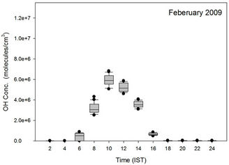


Figure 20. The diurnal variation pattern observed in the GEOS-Chem generated OH radical concentrations (molecules/cm3) for the co-ordinates (26˚N, 75˚E) for different months of the year 2009 at the ground level (0 - 0.3 km AGL).
transport on the measured SO2 values over Mt. Abu, GEOS-Chem model runs were performed with all the parameters keeping identical to the previous runs but now with the Transport mechanism turned OFF. Now the percentage difference in the SO2 concentration at 26˚N, 75˚E—the nearest grid point co-ordinates available with the GEOS-Chem model at 4˚ × 5˚ resolutions in the absence of transport is calculated as follows:
Percent Difference in the SO2 Concentration in the Absence of Transport = (WithOutTransport – FullInput) × 100/FullInput
where:
WithOutTransport → SO2 concentration recorded when the Transport turned OFF
FullInput → SO2 concentration recorded when Transport also was kept ON
Figure 22 shows the percent difference in the SO2 concentration in the absence of the transport mechanism over the co-ordinates (26˚N, 75˚E). Once the transport is turned OFF, sources located within the 4˚ × 5˚ grid containing

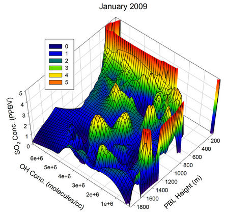
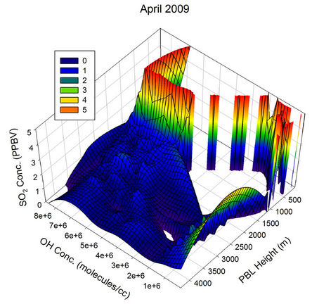
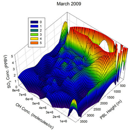

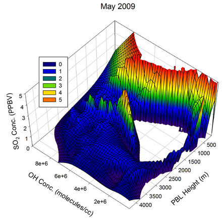
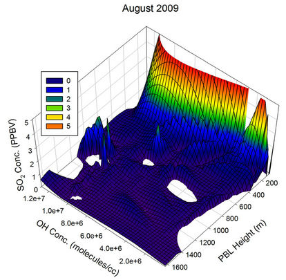
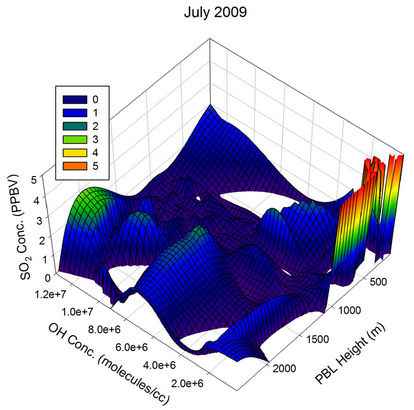
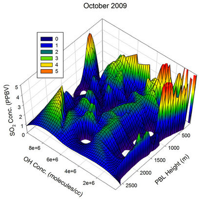
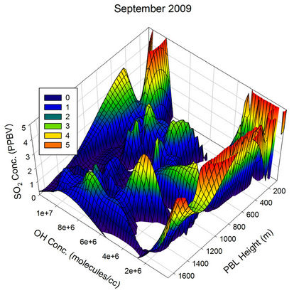
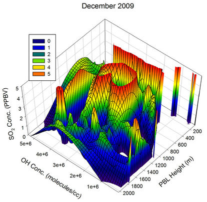

Figure 21. Three dimensional graphs showing the SO2 concentration dependence on the OH radical levels (molecules/cm3) and PBL heights (m) for different months of the year 2009. The time series SO2, OH and PBL heights were obtained from the GEOS-Chem model for the co-ordinates 26˚N, 75˚E.

Figure 22. Percent difference in the SO2 concentration in the absence of transport, for different months of the year 2009 calculated using GEOS-Chem model for the co-ordinates (26˚N, 75˚E) at the ground level (0 - 0.3 km AGL).
the Mt. Abu site only contribute to the observed SO2 levels.
It is found that in the absence of transport, there in a decrease in the SO2 levels during all the months, but with varying magnitude. The months Jan, Feb, Mar, and Apr receives the minimum contribution from long range transport while Jul and Dec sees the highest long range contribution to the ambient SO2 levels. The rest of the months receive intermediate contribution.
4. Conclusions
The SO2 measurements at the semi arid high altitude site, Gurushikhar, Mt. Abu (24.6˚N, 72.7˚E, 1680 m ASL), during Sept-Dec 2009 and Feb-Mar 2010 showed strong influences of long range transport from a source region surrounding 30˚N, 75˚E—the one with the highest SO2 concentration in the GEOS-Chem generated plots for the region and located in the vicinity of the sampling site— on the ambient SO2 levels over this region. The observed spikes in the measured SO2 spectra for the different sampling periods could be well explained by correlating the wind back trajectories with the GEOS-Chem generated SO2 plots for the entire region, viz. the spikes were present when the back trajectories extended to the high SO2 regions in the GEOS-Chem generated profiles.
During Sep-Oct 2009, when the wind back trajectories originated mostly from Arabian Sea, the SO2 concentration measured at Mt. Abu showed a near continuum with very few spikes. The minimal diurnal variability during this period is attributed to the entry of the high altitude sampling site to the free troposphere due to the low PBL heights for this month. During Nov 2009, the back trajectories showed pollutant transport from the high SO2 region located around 30˚N, 75˚E as well as low SO2 source regions in the GEOS-Chem generated SO2 profiles. The three short duration high magnitude spikes recorded each on 2nd (around 0125 hrs) 4th (around 2230 hrs) and 5th (around 2120 hrs) Nov 2009 were found to be associated with the plume transport from a major oil fire erupted at an IOCL depot in Jaipur (26.92˚N, 75.82˚E), located only a few co-ordinates away.
In Dec 2009, the winds were mostly from North and North-East occasionally carrying high SO2 from the source regions surrounding 30˚N, 75˚E causing many spikes in the SO2 spectra. The sampling period in Feb 2010 saw higher SO2 values and the clear diurnal variability for this month is attributed to the large diurnal PBL height variation. During Mar 2010 also, high SO2 concentrations were recorded and the well defined diurnal variability pattern is attributed again to the very large diurnal variability in the PBL heights.
The diurnal variation pattern in the measured SO2 spectra over Mt. Abu as well as those in the GEOS-Chem generated SO2 time series data were further systematically studied using the time series PBL height and OH radical values from the GEOS-Chem model, which showed these parameters significantly influencing the diurnal pattern of SO2 with a pronounced seasonality.
A separate study employing the GEOS-Chem model to understand the possible effects of long range transport on the SO2 levels over Mt. Abu showed a decrease in the SO2 levels in the absence of transport during all the months of the year with Jan, Feb, Mar, and Apr receiving the minimum contribution from long range transport while Jul and Dec receiving the maximum.
5. Acknowledgements
The ISRO-Geosphere Biosphere Program (Department of Space, Government of India) is acknowledged for the partial financial support for this study. The author is highly grateful to Prof. M. M. Sarin, Physical Research Laboratory, India, for the invaluable scientific discussions and support towards this study.
REFERENCES
- J. Crawford, J. Olson, D. Davis, et al., “Clouds and Trace Gas Distributions during TRACE-P,” Journal of Geophysical Research, vol. 108, No. D21, 2003, pp. 8818- 8830. doi:10.1029/2002JD003177
- T. Larssen, E. Lydersen, D. Tang, et al., “Acid Rain in China,” Environmental Science & Technology, Vol. 40, No. D2, 2006, pp. 418-425.
- T. Ohara, H. Akimoto, J. Kurokawa, et al., “An Asian Emission Inventory of Anthropogenic Emission Sources for the Period 1980-2020,” Atmospheric Chemistry and Physics Discuss, Vol. 7, 2007, pp. 4419-4444. doi:10.5194/acpd-7-6843-2007
- D. G. Streets, T. C. Bond, G. R. Carmichael, et al., “An Inventory of Gaseous and Primary Aerosol Emissions in Asia in the Year 2000,” Journal of Geophysical Research, Vol. 108, No. D21, 2003, pp. 8809-8831. doi:10.1029/2002JD003093
- D. G. Streets and S. T. Waldhoff, “Present and Future Emissions of Air Pollutants in China: SO2, NOX, and CO,” Atmospheric Environment, Vol. 34, No. 3, 2000, pp. 363-374. doi:10.1016/S1352-2310(99)00167-3
- T. Francis, “Effect of Asian Dust Storms on the Ambient SO2 Concentration over North-East India: A Case Study,” Journal of Environmental Protection, Vol. 2, No. 6, 2011, pp. 778-795. doi:10.4236/jep.2011.26090
- D. C. Thornton, A. R. Bandy, B. W. Blomquist, et al., “Sulfur Dioxide as a Source of Condensation Nuclei in the Upper Troposphere of the Pacific Ocean,” Journal of Geophysical Research, Vol. 101, No. D1, 1996, pp. 1883 -1890. doi:10.1029/95JD02273
- D. C. Thornton, A. R. Bandy, B. W. Blomquist, et al., “Transport of Sulfur Dioxide from the Asian Pacific Rim to the North Pacific Troposphere,” Journal of Geophysical Research, Vol. 102, No. D23, 1997, pp. 28489-28499. doi:10.1029/97JD01818
- C. M. Benkovitz, M. T. Scholtz, J. Pacyna, et al., “Global gridded Inventories of Anthropogenic Emissions of Sulfur and Nitrogen,” Journal of Geophysical Research, Vol. 101, No. D22, 1996, pp. 29239-29253. doi:10.1029/96JD00126
- P. A. Spiro, D. J. Jacob and J. A. Logan, “Global Inventory of Sulfur Emissions with 1˚ × 1˚ Resolution,” Journal of Geophysical Research, Vol. 97, No. D5, 1992, pp. 6023-6036. doi:10.1029/91JD03139
- M. O. Andreae, “Ocean-Atmosphere Interactions in the Global Biogeochemical Sulfur Cycle,” Marine Chemistry, vol. 30, 1990, pp. 1-29. doi:10.1016/0304-4203(90)90059-L
- M. O. Andreae and W. A. Jaeschke, “Exchange of Sulfur between Biosphere and Atmosphere over Temperate and Tropical Regions,” In: R. W. Howarth and J. W. B. Stewart, eds., Sulfur Cycling in Terrestrial Systems and Wetlands, John Wiley, New York, 1992.
- T. S. Bates, J. D. Cline, R. H. Gammon, et al., “Regional and Seasonal Variations in the Flux of Oceanic Dimethyl Sulfide to the Atmosphere,” Journal of Geophysical Research, Vol. 92, No. C3, 1987, pp. 2930-2938. doi:10.1029/JC092iC03p02930
- C. F. Cullis and M. M. Hirschler, “Atmospheric Sulphur: Natural and Man-Made Sources,” Atmospheric Environment, vol. 14, No. 11, 1980, pp. 1263-1278.
- J. R. Freney, M. V. Ivanov and H. Rhodhe, “The Sulphur Cycle, in the Major Biogeochemical Cycles and Their Interactions, SCOPE 24,” John Wiley, New York, 1983.
- H. Rodhe and I. Isaksen, “Global Distribution of Sulfur Compounds in the Troposphere Estimated in a Height/ Latitude Transport Model,” Journal of Geophysical Research, Vol. 85, No. C12, 1980, pp. 7401-7409. doi:10.1029/JC085iC12p07401
- E. S. Saltzman and D. J. Cooper, “Shipboard Measurements of Atmospheric Dimethyl Sulfide and Hydrogen Sulfide in the Caribbean and Gulf of Mexico,” Journal of Atmospheric Chemistry, vol. 7, No. 2, 1988, pp. 191-209. doi:10.1007/BF00048046
- O. B. Toon, et al., “The Sulfur Cycle in the Marine Atmosphere,” Journal of Geophysical Research, Vol. 92, No. D1, 1987, pp. 943-963. doi:10.1029/JD092iD01p00943
- L. Gerhardsson, A. Oskarsson and S. Skerfving, “Acid Precipitation—Effects on Trace Elements and Human Health,” The Science of the Total Environment, vol. 153, No. 3, 1994, pp. 237-245. doi:10.1016/0048-9697(94)90203-8
- D. W. Schindler, “Effects of Acid Rain on Freshwater Ecosystems,” Science, vol. 239, No. 4836, 1988, pp. 149- 157.
- Y. Igarashi, Y. Sawa, K. Yoshioka, et al., “Monitoring the SO2 Concentration at the Summit of Mt. Fuji and a Comparison with Other Trace Gases during Winter,” Journal of Geophysical Research, Vol. 109, No. D17, 2004, Article ID D17304. doi:10.1029/2003JD004428
- W. T. Luke, “Evaluation of a Commercial Pulsed Fluorescence Detector for the Measurement of Low-Level SO2 Concentrations during the Gas-Phase Sulfur Intercomparison Experiment,” Journal of Geophysical Research, Vol. 102, No. D13, 1997, pp. 16255-16265. doi:10.1029/96JD03347
- M. Luria, J. F. Boatman, J. Harris, et al., “Atmospheric Sulfur Dioxide at Mauna Loa, Hawaii,” Journal of Geophysical Research, Vol. 97, No. D5, 1992, pp. 6011-6022. doi:10.1029/91JD03126
- I. Bey, D. J. Jacob, R. M. Yantosca, et al., “Global Modeling of Tropospheric Chemistry with Assimilated Meteorology: Model Description and Evaluation,” Journal of Geophysical Research, Vol. 106, No. D19, 2001, pp. 23073-23095. doi:10.1029/2001JD000807
- R. J. Park, D. J. Jacob, B. D. Field, et al., “Natural and Transboundary Pollution Influences on Sulfate-NitrateAmmonium Aerosols in the United States: Implications for Policy,” Journal of Geophysical Research, Vol. 109, No. D15, 2004, Article ID D15204. doi:10.1029/2003JD004473
- J. Wang, D. J. Jacob and S. T. Martin, “Sensitivity of Sulfate Direct Climate Forcing to the Hysteresis of Particle Phase Transitions,” Journal of Geophysical Research, Vol. 113, No. D11, 2008, Article ID D11207. doi:10.1029/2007JD009368
- T. Duncan Fairlie, D. J. Jacob and R. J. Park, “The Impact of Transpacific Transport of Mineral Dust in the United States,” Atmospheric Environment, vol. 41, No. 6, 2007, pp. 1251-1266. doi:10.1016/j.atmosenv.2006.09.048
- D. Chen, Y. Wang, M. B. McElroy, et al., “Regional CO Pollution and Export in China Simulated by the HighResolution Nested-Grid GEOS-Chem Model,” Atmospheric Chemistry and Physics, vol. 9, No. 11, 2009, pp. 3825-3839. doi:10.5194/acp-9-3825-2009
- V. Vestreng and H. Klein, “Emission Data Reported to UNECE/EMEP. Quality Assurance 769 and Trend Analysis and Presentation of WebDab,” MSC-W Status Report, Norwegian Meteorological Institute, 2002.
- H. Kuhns, M. Green and V. Etyemezian, “Big Bend Regional Aerosol and Visibility Observational (BRAVO) Study Emissions Inventory,” Desert Research Institute, 2003.
- J. G. J. Olivier and J. J. M. Berdowski, “Global Emissions Sources and Sinks, in the Climate System,” The Netherlands A.A. Balkema Publishers/Swets & Zeitlinger Publishers, 2001.
- D. G. Streets, Q. Zhang, L. Wang, et al., “Revisiting China’s CO Emissions after the Transport and Chemical Evolution over the Pacific (TRACE-P) Mission: Synthesis of Inventories, Atmospheric Modeling, and Observations,” Journal of Geophysical Research, Vol. 111, No. D14, 2006, Article ID D14306. doi:10.1029/2006JD007118
- R. R. Draxler and G. D. Rolph, “HYSPLIT—HYbrid Single-Particle Lagrangian Integrated Trajectory Model,” 2012. http://www.arl.noaa.gov/ready/hysplit4.html
- G. D. Rolph, “Real-Time Environmental Applications and Display System (READY),” 2003.