Atmospheric and Climate Sciences
Vol.3 No.4(2013), Article ID:37124,9 pages DOI:10.4236/acs.2013.34055
Stable Boundary Layer Height Parameterization: Learning from Artificial Neural Networks
Department of Marine, Earth, and Atmospheric Sciences, North Carolina State University, Raleigh, USA
Email: misswindy78@gmail.com
Copyright © 2013 Wei Li. This is an open access article distributed under the Creative Commons Attribution License, which permits unrestricted use, distribution, and reproduction in any medium, provided the original work is properly cited.
Received May 17, 2013; revised June 18, 2013; accepted June 26, 2013
Keywords: Artificial Neural Network; Large-Eddy Simulation; Stable Boundary Layer Height
ABSTRACT
Artificial neural networks (ANN) are employed using different combinations among the surface friction velocity u*, surface buoyancy flux Bs, free-flow stability N, Coriolis parameter f, and surface roughness length z0 from large-eddy simulation data as inputs to investigate which variables are essential in determining the stable boundary layer (SBL) height h. In addition, the performances of several conventional linear SBL height parameterizations are evaluated. ANN results indicate that the surface friction velocity u* is the most predominant variable in the estimation of SBL height h. When u* is absent, the secondly important variable is the surface buoyancy flux Bs. The relevance of N, f, and z0 to h is also discussed; f affects more than N does, and z0 shows to be the most insensitive variable to h.
1. Introduction
Parameterizations of the stable boundary layer (SBL) height are often critical in many practical problems, such as air pollutant dispersion modeling [1-3], weather modeling, and climate modeling. Due to the complex relationship between the mean profiles and the turbulence in the stable boundary layer [4,5], it is less straightforward to determine the SBL height from wind speed and temperature profiles compared to observing the convective boundary layer height from mean profiles. During recent several decades, a number of model formulations of SBL depth have been developed based on various datasets [6-11]; these formulations are mainly in forms of linear equations or complex non-linear multi-limit equations. Most of these schemes are surface flux-dominated models; they are summarized by Zilitinkevich et al. [11].
Various linear relationships [6-8] were formulated by considering the SBL height relying on one or two variables among the earth’s rotation (f), surface friction velocity (u*), surface buoyancy flux (Bs), and free-flow stability (N) which have been identified as the key physical processes that govern the SBL height. However, no consensus was achieved from these linear models.
By employing the turbulent kinetic energy (TKE) budget equation, Zilitinkevich and Mironov [10] derived two diagnostic multi-limit equations for the equilibrium depth of SBL that contains all the four aforementioned variables and several unknown coefficients, and that can hold in both the general case and the limiting cases. Furthermore, Zilitinkevich et al. [11] proposed two refined Ekman-layer height equations from the momentum balance equations and validated their model against observations.
The above parameterizations of SBL height have been evaluated by many researchers based on various observational datasets [11-14] and controlled numerical simulations [15-17]. Using datasets over grassland, cooler ocean surface and snow cover, Vickers and Mahrt [13] evaluated a variety of surface flux-based SBL height formulations; they summarized that the existing formulations generally perform poorly and often overestimate the depth of SBL.
The aforementioned multi-limit equations were further discussed and evaluated by Zilitinkevich and Baklanov [12]; they found that the Ekman-layer height equations by Zilitinkevich et al. [11] produced more accurate estimation of SBL height than that by the equations in Zilitinkevich and Mironov [10]. Kosovic and Lundquist [17] compared several parameterizations to calculate SBL height using large-eddy simulations of moderately stable boundary layers and they demonstrated that the gravity waves in the free atmosphere do affect the height of SBL.
Steeneveld et al. [14] evaluated the performance of the Zilitinkevich and Mironov [10] multi-limit equations against four observational datasets over different terrains; they found that the multi-limit equations underestimate the SBL height, especially for shallow boundary layers, and no unique parameter that sets for these equations can be determined. Alternatively, Steeneveld et al. [14] developed a formulation based on formal dimensional analysis using the same quantities as in the multi-limit equations; this new formulation showed to be more robust and it significantly reduced the model bias for shallow boundary layer heights compared with the multi-limit equations, and a unique parameter set was found for this new equation. Furthermore, Steeneveld et al. [18] proposed another alternative equation by an inverse interpolation of the eddy diffusivities for each boundary layer prototype [16] instead of interpolating the height scales for each prototype in the equations by Zilitinkevich and coworkers when applying the definition of Ekman layer depth. This equation reduced the bias of the predicted SBL height compared to their equations. However, the formulation derived from formal dimensional analysis [14] still shows better performance than this equation [18].
Therefore, the above studies have enlightened us that some formulations which involve less variables can perform better than the complex multi-limit formulations for the SBL height estimation. In this paper, we will take an unconventional approach to figure out which variables are indeed essential for an optimum representation of the SBL height. Artificial neural networks will be employed to model this non-linear phenomenon based on a largeeddy simulation output dataset.
2. Data Description
The data used in this study are the output from 68 runs of large eddy simulation (LES). They are idealized simulations, by setting different values for the parameters of geostrophic wind G, cooling rate C of air temperature, surface roughness length z0, initial boundary layer height H, Brunt-Vaisala frequency N in the free atmosphere above the SBL, and Coriolis parameter f, to represent typical low-level jet scenarios in the stable boundary layer.
The LES computational domain employed for this study extends 800 meters in the lateral direction and 795 meters in the vertical direction. The grid size in both y and z directions is 10 meters; at each grid point, the three dimensional wind velocity and air temperature are generated as a time series; the time step for the LES flow fields is 0.1 sec [19]. The 5-min mean values of the simulated data are output for the boundary layer height studies. From each LES run, a total of 144 time steps are obtained representing 12 hours of simulation between 1800 to 0600 LST.
Each simulation starts from a neutral profile. As shown by the wind profiles, the damping layer of wind speed starts from 550-m level around, we only use the data from the surface to 550-m height to analyze the stable boundary height.
There have been many definitions of SBL height with different emphasis on properties of turbulence [20], heat flux [21], mean wind speed [22], mean temperature [23], and other effects [16,24,25]. In this study, we will employ the definition of the height of the lowest maximum of the wind speed [22,26], often referred to as the lowlevel jet height, as the targeted SBL height h in the parameterization. The LES wind profiles show that low-level jets usually start developing after 0000 LST. Therefore, only the data between 0000 - 0600 LST in each simulation are selected to represent typical low-level jets.
3. Resampling Strategy
In this study, at each time step in each LES run, from the wind speed profile, a SBL height h can be estimated as the height of the maximum wind speed, i.e., the low-level jet height. Thus from each simulation there are totally 72 output values of 6 hours for surface friction velocity u*, surface buoyancy flux Bs, and boundary layer height h. The geostrophic wind G, the Coriolis parameter f, the Brunt-Vaisala frequency N in the free atmosphere, and the surface roughness length z0 are set as various values for each LES run.
We will firstly combine the data from all the 68 LES sruns together to form a total dataset, and then apply repeated random sub-sampling cross-validation algorithm, to evaluate five conventional linear formulations of stable boundary layer height. This method randomly partitions the dataset into training and validation data by a certain percentage (60% training and 40% validation in this study). For each such split, the model is fit to the training data, and assesses the predictive accuracy using the validation data. This procedure is repeated for 100 times in this study.
The variables from the training data are used in the conventional linear formulations to calculate their included constants first. Then substituting the variables in the validation data, together with the derived constants into the linear equations, the SBL height h can be predicted. Consequently based on the difference between the predicted and the targeted values of h, the statistical quantities such as root mean squared error (RMSE), median absolute error (MAE), median bias error (MBE), and index of agreement (IOA) are calculated. Therefore the performance of these linear formulations can be evaluated from the distribution of the statistical errors.
4. Performance of Conventional SBL Height Parameterizations Based on LES Data
Most conventional formulations for the equilibrium depth of the stably stratified boundary layer are surfaceflux-dominated formulations. In these parameterizations, the turbulent heat flux and momentum flux at the surface are required to be estimated. Rossby and Montgomery [27] proposed that the surface friction velocity u* and Coriolis parameter f mainly affect the stable boundary layer depth:
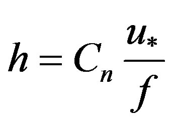 (1)
(1)
Then Zilitinkevich [7] considered the surface heat flux together with the influences of surface friction and the earth’s rotation such that
 (2)
(2)
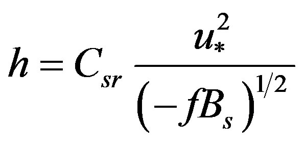
where Bs is the surface buoyancy flux. Pollard et al. [8] were the first to suggest that N, the free-flow stratification above the stable boundary layer, would affect the boundary layer height:
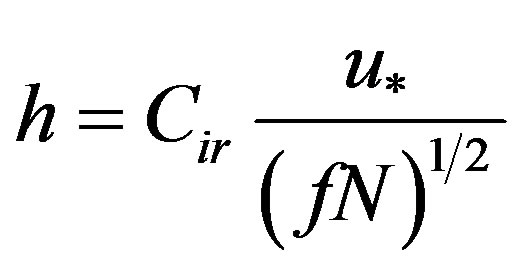 (3)
(3)
Kitaigorodskii [6] proposed that only the surface heat flux and momentum flux are dominated on the depth of the boundary layer without the effect of earth rotation
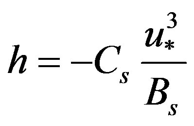 (4)
(4)
When only considering surface momentum flux and the overlying free-flow stratification, Kitaigorodskii and Joffre [9] obtained
 (5)
(5)
In this study, we evaluate the performance of the above five parameterizations against controlled large eddy simulation output. Figure 1 shows the statistical errors of RMSE, MAE, MBE, and IOA between the predicted and the target values of stable boundary layer
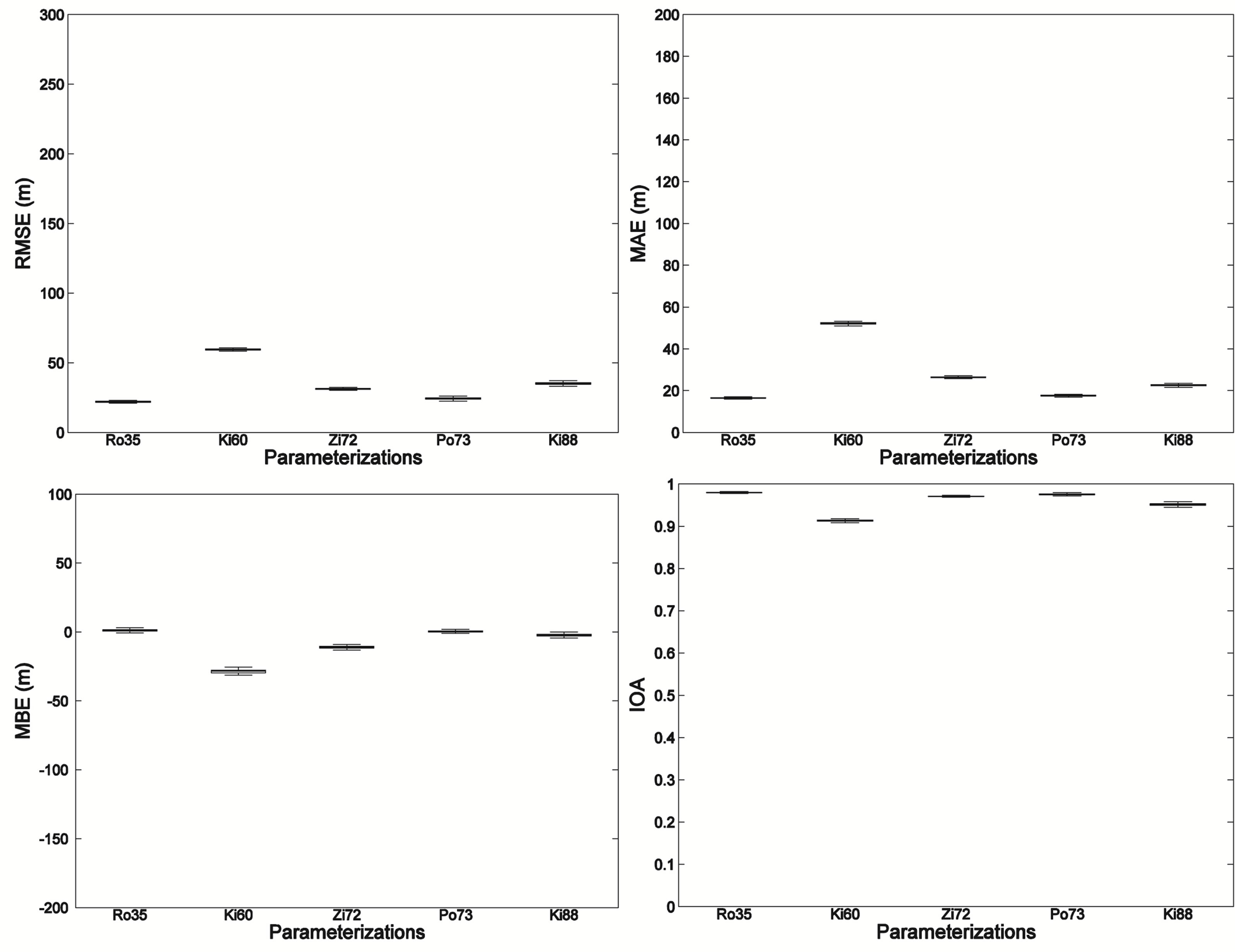
Figure 1. Performance of conventional linear parameterizations.
height h based on these five formulations.
The formulation by Rossby and Montgomery [27] when only considering influences of u* and f shows the best performance with minimum values of RMSE (25 m) and MAE (18 m) among others. The Pollard et al. [8] scheme performs secondly best with a RMSE of 30 m and a MAE of 20 m when N is taken into account. Then Zilitinkevich [7] formulation has slightly larger RMSE than that by Pollard et al. [8] when N is replaced by Bs. When f is not involved in the formulations [Equations (4) and (5)], the models biases are largely increased with Equation (4) being the worst case.
Therefore, the performance of these conventional linear parameterizations of SBL height against LES data indicates that the surface friction velocity u* and Coriolis parameter f are proved to be the two most predominant variables to determine h and the free-flow stability N shows more important than the surface buoyancy flux Bs.
5. Artificial Neural Networks
Artificial neural networks (ANN) are composed of simple interconnected neurons. Unlike other statistical techniques, ANN usually makes no prior assumptions regarding the data distribution, and can model extremely non-linear relationships and be trained to be accurately representative for new and unseen data [28]. Typically, a neural network can be trained based on a comparison between the output and the target until the network output matches the target, so that a particular input leads to a specific target output.
Artificial neural networks have been applied to perform complex functions in various fields. In recent years, a significant number of ANN applications have been developed in different fields of geosciences such as satellite remote sensing, meteorology, oceanography, numerical weather prediction, and climate studies [29].
The work flow for the general neural network design process has the following three primary steps:
5.1. Collect and Prepare the Data
After the sample data have been collected, they need to be preprocessed and to be divided into three subsets before they are used to train the network. The first subset is the training set, which is used for computing the gradient and updating the network weights and biases. The second subset is the validation data which will determine the stopping criteria. The error on the validation set is monitored during the training process. The validation error normally decreases during the initial phase of training, as does the training set error. However, when the network begins to over fit the data, the validation error typically begins to rise after some iterations. The network weights and biases are saved when the validation error reaches the minimum at the certain iteration, which gives the optimum iteration number for the network training. The third subset in the data is the testing data, the error on which is not used during the training process, but used to compare different models. Typically, a poor division of the dataset happens when the testing error reaches a minimum at a significantly different iteration number from that at which the validation error reaches its minimum.
5.2. Create, Configure and Initialize the Network
After the data have been prepared, the next step is to select the network architecture and create the network. In this paper, the most predominant network architecture of multilayer perceptron is utilized to map the relationships between the stable boundary layer height h and the associated variables u*, Bs, N, f, and z0. We create a two-layer feedforward network (see Figure 2). The sum of the weighted inputs and the bias forms the input to the transfer function in the network; then the transfer function generates the output vector [28,30]. Multilayer networks often use the log-sigmoid transfer function.
After configuring the network object and also initializing the weights and biases of the network, the network is ready for training.
5.3. Train and Validate the Network
The process of training a neural network involves adjusting the values of the weights and biases of the network to optimize the network performance, that is, to find the combination of weights which can result in the smallest error [28]. The default performance function for feedforward networks is the mean square error (MSE) between the network outputs and the targets.
Gradient descent is the simplest optimization algorithm; the gradient is calculated using the technique of
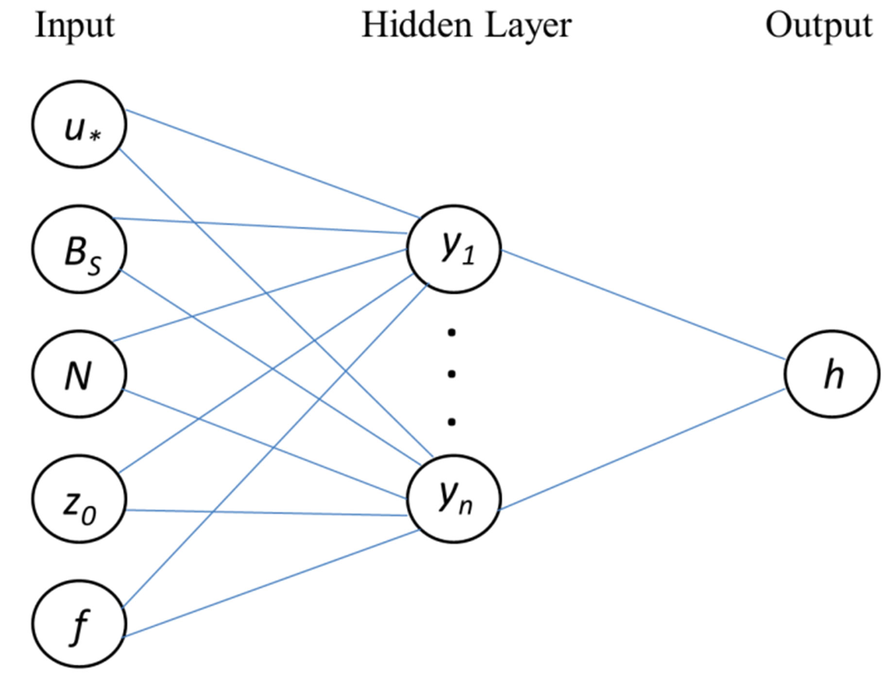
Figure 2. Illustration of the ANN architecture for modeling stable boundary layer height.
back propagation algorithm, which involves performing computations backward through the network and is the most computationally straightforward algorithm for training the multilayer perceptron [28,31]. The gradient descent algorithm updates the network weights and biases in the direction in which the performance function decreases most rapidly.
Once the training procedure is complete, the network validation can be done by checking the training record and creating a regression plot between the outputs of the network and the targets.
6. ANN Modeling Strategy of Stable Boundary Layer Height
In this study, we will apply ANN to predict the stable boundary layer height. ANN development for simulating the SBL height requires identification of the input and output variables. From the knowledge of conventional parameterizations, the SBL height h can be expressed as a function of surface friction velocity u*, surface buoyancy flux Bs, Brunt-Vaisala frequency N in the free atmosphere above the SBL, Coriolis parameter f, and surface roughness length z0.
Figure 2 shows the illustration of the two-layer perceptron ANN architecture in modeling the SBL height h. The architecture of the network depends on the number of input and output variables. For the present problem, the number of input nodes in the two-layer perceptron network varies from the minimum of 1 to the maximum of 5; the input variables are randomly combined among the five associated variables u*, Bs, N, f, and z0. Table 1 shows the 31 variable combinations of inputs used in the network. Only one output node exists in this problem.
However, the number of nodes in the hidden layer is not fixed. For each combination of input variables, we test the network by changing the neuron number in the hidden layer from 1 to 20 in turn to find a best number of hidden nodes. At each specific hidden nodes number, the network is repeated to run 100 times to calculate a statistical median value of the errors. For each run, the dataset are randomly partitioned into three subsets of training, validation, and testing data with the proportion of 30%, 30%, and 40%, respectively.
ANNs are developed using MATLAB Neural Network Toolbox (version 2010). The back propagation algorithm is applied for training. The training is performed using the default values for the parameters of the network.
7. Performance of ANN-Based Parameterizations Based on LES Data
From previous studies, the basic variables that govern the SBL height h are the surface friction velocity u*, the surface buoyancy flux Bs, the free-flow stability N, the
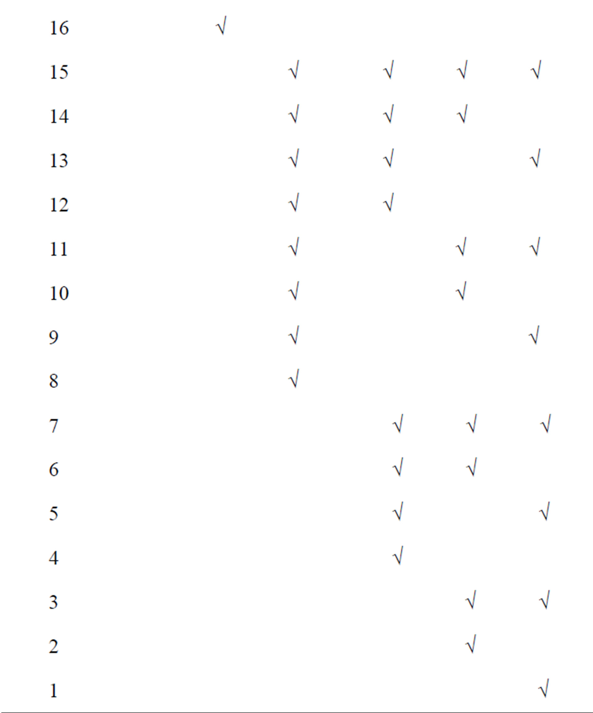
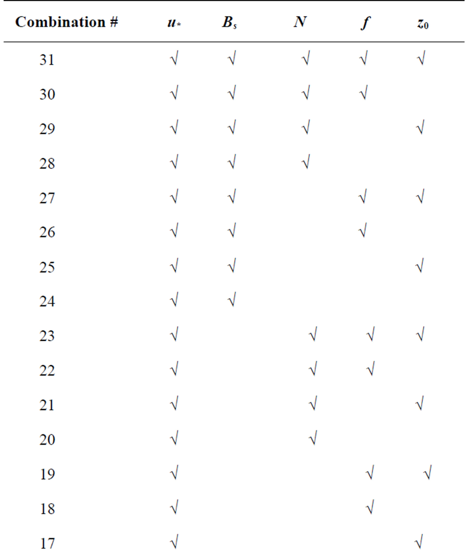
Table 1. Input variable combinations in ANN modeling.
Coriolis parameter f, and the surface roughness length z0. In this study, these five variables u*, Bs, N, f, and z0 were randomly combined into 31 different combinations of inputs for the neural network in the order of binary numbers (see Table 1) to investigate which combination of variables is the optimum input in determining the stable boundary layer height h. Figure 3 shows the statistical errors of RMSE, MAE, MBE, and IOA calculated between the output value and the target value of SBL height h in the network based on the 31 input combinations utilizing the LES output data.
We divided the 31 combinations into 4 groups. From the first group of combinations (combination number 1 to 7 in Table 1) where the variables u* and Bs are not involved in the input, the model performance is very poor. The values of RMSE are as high as 75 m; all the IOA values are lower than 0.3.
In the second group of combinations (combination number 8 to 15 in Table 1), when the surface buoyancy flux Bs are included in the model input, the RMSE decrease to be around 50 m, the IOA are largely increased up to 0.9. This indicates that buoyancy flux is a very important variable in predicting h when friction velocity is absent in the input.
When the third (combination number 16 to 23 in Table 1) and the fourth (number 24 to 31) groups of combinations are input into the network, where the surface friction velocity u* is involved in each input, the model performance is largely improved again to be the best among all the variable combinations of input. The RMSE are very close to each other based on these 16 set of inputs, with a mean value of 20 m, and their IOA reach to be as high as 0.98. This strongly proves that the surface friction velocity u* is the most dominant variable in determining the SBL height.
From the second group to the fourth group of variable combinations, keeping the way of combining other three variables (N, f, z0) as that in the first group, when adding u* with Bs in the input variables, the model performance is largely improved. From the second group to the third group, when Bs is replaced by u* in the input, the model performance is largely improved similarly. This indicates that the variable Bs has less relevance compared to u* in predicting h, even if Bs has been proved to be an important one. This can also be verified from that when changing the input combinations from the fourth group to the third group, where Bs is removed from the variable combinations, the model performance is not changed obviously.
The median RMSE based on the variable combination of (u*, Bs, N, f, z0) is the minimum of the RMSE values based on all combinations. This means that when all the
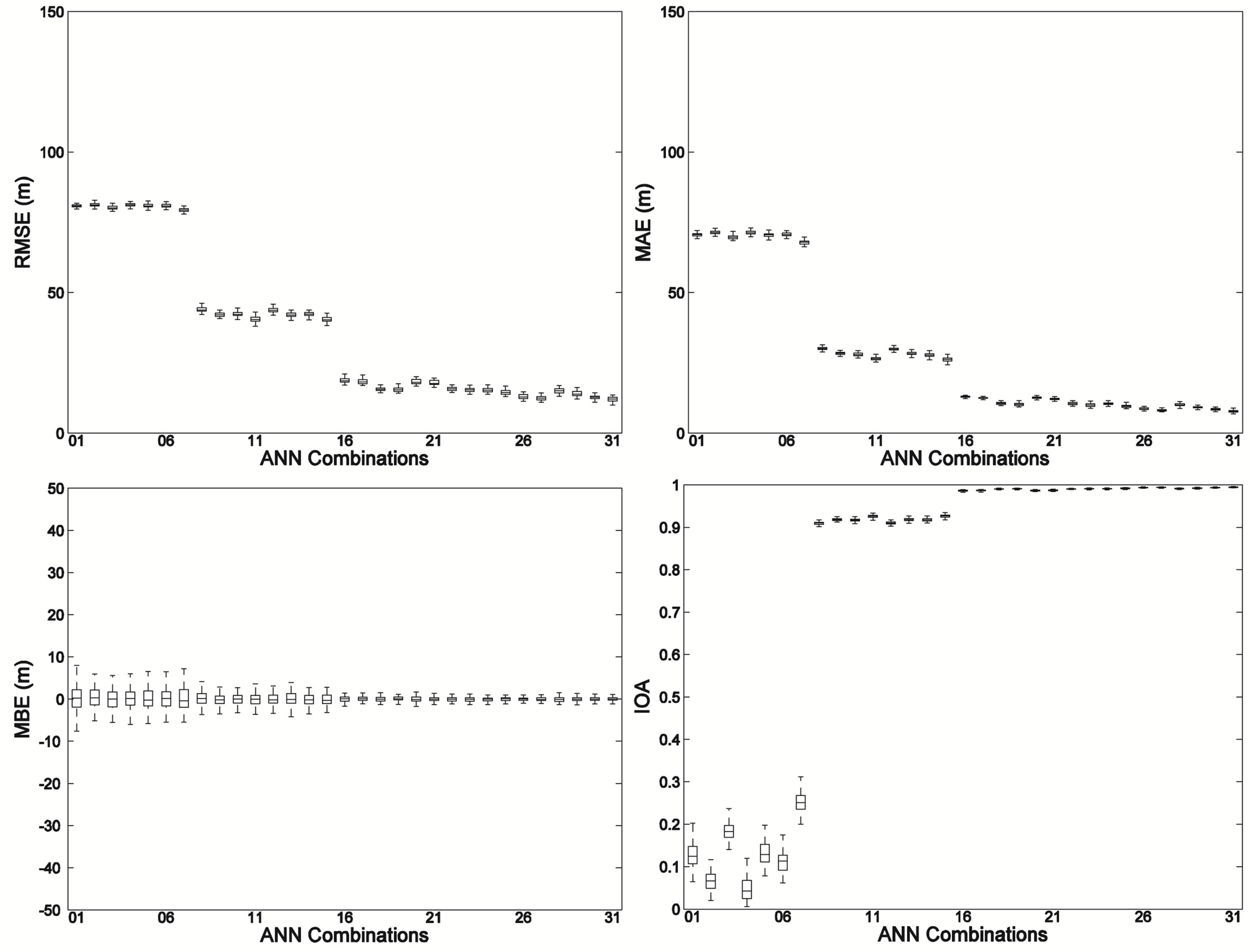
Figure 3. Performance of ANN-based parameterizations using 31 different variable combinations as inputs.
five relevant variables u*, Bs, N, f, and z0 are taken into account in the model input, the model performs best.
In addition, within the third and fourth groups, when the coriolis parameter f is added into the combinations, the RMSE values are decreased; when replacing f by N in the combinations, RMSE are increased; when f and N are both involved, the RMSE values are decreased again. Therefore, the coriolis parameter f shows to be more important for h prediction compared to the inversion strength N.
In further details, within both the third group and the fourth group, the values of RMSE are changing in pairs. The two median RMSE values of each pair are almost equal; the difference between the two input variable combinations within each pair is that the surface roughness length z0 is included or not. This demonstrates that the surface roughness length z0 is not obviously affective to h determination.
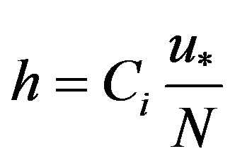
Overall, our results based on ANN shows that the strongest relation of h exists with u*, and then with Bs secondly. Koracin and Berkowicz [32] ever proposed a simple empirical estimate of h = 700u*. This formula was evaluated by Steeneveld et al. [14] by observational data and it performs well over their datasets. In the alternative formulation using dimensional analysis by Steeneveld et al. [14], they also concluded that h relies on u* most strongly, and then on Bs in the very stable limit, then on N while f and z0 are less relevant for their data; when the Coriolis parameter f is omitted, the SBL height h for moderately stable conditions is proportional to u*/N, and for high stability conditions h is proportional to the length scale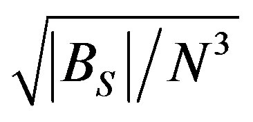 .
.
Kosovic and Lundquist [17] also used LES study to explore various parameterizations of SBL height. They found that from a small-domain simulation, the SBL height formulation proposed by Kosovic and Curry [15] in which the strength of the inversion N was not involved (except for u*, Bs and f) appeared to match the SBL height defined by turbulent shear stress better than the scheme by Zilitinkevich et al. [11] did in which N was involved, due to the simulation domain was too small to include the effects of gravity waves that developed above the SBL. They also conducted medium-resolution LES with the domain size sufficiently large to resolve the overlying gravity waves; the results showed that the formulation [11] with N involved consequently gave a better prediction of SBL height.
In the conventional formulations, the friction velocity u* and Coriolis parameter f are proved to be the two most predominant variables in determining h, whereas the surface buoyancy flux Bs is not an important factor and even has less influence than the free-flow stability N. Table 2 compares the model performance given by the statistical errors of RMSE, MBE, MAE and IOA based
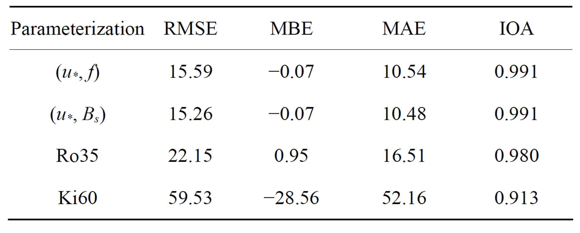
Table 2. Performance of two linear parameterizations and two ANN-based parameterizations using corresponding variable combinations as inputs.
on the conventional formula of h = Cnu*/f by Rossby and Montgomery [27] (Ro35 in Figure 1) and based on the input variable combination of (u*, f) in ANN. Their performance is quite good and they have close RMSE values of 22 m and 16 m; both have very high IOA values nearing to 1. The cases for the conventional formula h = −Csu*3/Bs by Kitaigorodskii [6] (Ki60 in Figure 1) and the variable combination of (u*, Bs) in ANN are also listed in Table 2. Although Ki60 results in a very high IOA value of 0.91, its RMSE is as large as 60 m, which is much larger than the RMSE of 15 m for the combination (u*, Bs) in ANN. As discussed in section 4, this Ki60 formulation performs worst among the five conventional formulations (Figure 1); this might be due to the cube of u* in the formulation and needs to be further explored.
8. Conclusions
In this paper, we tried to find out which variables are essential and can achieve the best performance in determining the stable boundary layer height h based on largeeddy simulation data. Artificial neural networks were applied to investigate which combination of variables is the optimum input. We also evaluated the performance of conventional linear formulations for the SBL height prediction, in which the surface friction velocity u* and the Coriolis parameter f were proved to be the two most predominant variables to determine h and the free-flow stability N showed to be more important than the surface buoyancy flux Bs for h prediction.
The results based on ANN showed that the strongest relation of h exists with the surface friction velocity u*. The secondly dominant variable relevant to h is the surface buoyancy flux Bs. The Coriolis parameter f shows to be more important compared to the inversion strength N. The surface roughness length z0 is not an affective variable to h.
9. Acknowledgements
We thank Dr. Sukanta Basu in the Department of Marine, Earth, and Atmospheric Sciences at North Carolina State University for providing the LES dataset and codes in this study.
REFERENCES
- P. Seibert, F. Beyrich, S. E. Gryning, S. Joffre, A. Rasmussen and P. H. Tercier, “Review and Intercomparison of Operational Methods for the Determination of the Mixing Height,” Atmospheric Environment, Vol. 34, No. 7, 2000, pp. 1001-1027. http://dx.doi.org/10.1016/S1352-2310(99)00349-0
- J. A. Salmond and I. G.McKendry, “A Review of Turbulence in the Very Stable Boundary Layer and Its Implications for Air Quality,” Progress in Physical Geography, Vol. 29, No. 2, 2005, pp. 171-188. http://dx.doi.org/10.1191/0309133305pp442ra
- G. J. Steeneveld and A. A. M. Holtslag, “Meteorological Aspects of Air Quality,” Air Quality in the 21st Century, Nova Science Publishers, New York, 2009, pp. 67-114.
- W. Brutsaert, “Radiation, Evaporation and the Maintenance of the Turbulence under Stable Conditions in the Lower Atmosphere,” Boundary-Layer Meteorology, Vol. 2, No. 3, 1972, pp. 309-325. http://dx.doi.org/10.1007/BF02184772
- L. Mahrt, “Modeling the Height of the Stable Boundary Layer,” Boundary-Layer Meteorology, Vol. 21, No. 1, 1981, pp. 3-19. http://dx.doi.org/10.1007/BF00119363
- S. A. Kitaigorodskii, “On the Computation of the Thickness of the Wind-Mixing Layer in the Ocean,” Izvestiya AN SSSR, Geophysical Series, Vol. 3, 1960, pp. 425-431.
- S. S. Zilitinkevich, “On the Determination of the Height of the Ekman Boundary Layer,” Boundary-Layer Meteorology, Vol. 3, No. 2, 1972, pp. 141-145. http://dx.doi.org/10.1007/BF02033914
- R. T. Pollard, P. B. Rhines and R. Thompson, “The Deepening of the Wind-Mixed Layer,” Geophysical Fluid Dynamics, Vol. 3, 1973, pp. 381-404.
- S. A. Kitaigorodskii and S. M. Joffre, “In Search of Simple Scaling for the Heights of the Stratified Atmospheric Boundary Layer,” Tellus, Vol. 40A, No. 5, 1988, pp. 419- 443. http://dx.doi.org/10.1111/j.1600-0870.1988.tb00359.x
- S. S. Zilitinkevich and D. V. Mironov, “A Multi-Limit Formulation for the Equilibrium Depth of a Stably Stratified Boundary Layer,” Boundary-Layer Meteorology, Vol. 81, No. 3-4, 1996, pp. 325-351. http://dx.doi.org/10.1007/BF02430334
- S. S. Zilitinkevich, A. Baklanov, J. Rost, A. S. Smedman, V. Lykosov and P. Calanca, “Diagnostic and Prognostic Equations for the Depth of the Stably Stratified Ekman Boundary Layer,” Quarterly Journal of the Royal Meteorological Society, Vol. 128, No. 1, 2002, pp. 25-46. http://dx.doi.org/10.1256/00359000260498770
- S. S. Zilitinkevich and A. Baklanov, “Calculation of the Height of Stable Boundary Layers in Practical Applications,” Boundary-Layer Meteorology, Vol. 105, No. 3, 2002, pp. 389-409. http://dx.doi.org/10.1023/A:1020376832738
- D. Vickers and L. Mahrt, “Evaluating Formulations of the Stable Boundary Layer Height,” Journal of Applied Meteorology, Vol. 43, No. 11, 2004, pp. 1736-1749. http://dx.doi.org/10.1175/JAM2160.1
- G. J. Steeneveld, B. J. H. Van de Wiel and A. A. M. Holtslag, “Diagnostic Equations for the Stable Boundary Layer Height: Evaluation and Dimensional Analysis,” Journal of Applied Meteorology and Climatology, Vol. 46, No. 2, 2007, pp. 212-225. http://dx.doi.org/10.1175/JAM2454.1
- B. Kosovic and J. A. Curry, “A Large Eddy Simulation Study of a Quasi-Steady, Stably Stratified Atmospheric Boundary Layer,” Journal of the Atmospheric Sciences, Vol. 57, No. 8, 2000, pp. 1052-1068. http://dx.doi.org/10.1175/1520-0469(2000)057<1052:ALESSO>2.0.CO;2
- S. S. Zilitinkevich and I. Esau, “The Effect of Baroclinicity on the Equilibrium Depth of Neutral and Stable Planetary Boundary Layers,” Quarterly Journal of the Royal Meteorological Society, Vol. 129, No. 595, 2003, pp. 3339-3356. http://dx.doi.org/10.1256/qj.02.94
- B. Kosovic and J. K. Lundquist, “Influences on the Height of the Stable Boundary Layer,” 16th Symposium on Boundary Layers and Turbulence, American Meteor Society, Portland, 23 June 2004, Preprints.
- G. J. Steeneveld, B. J. H. Van de Wiel and A. A. M. Holtslag, “Notes and Correspondence: Comments on Deriving the Equilibrium Height of the Stable Boundary Layer,” Quarterly Journal of the Royal Meteorological Society, Vol. 133, No. 622, 2007, pp. 261-264. http://dx.doi.org/10.1002/qj.26
- C. Sim, S. Basu and L. Manuel, “On Space-Time Resolution of Inflow Representations for Wind Turbine Loads Analysis,” Energies, Vol. 5, No. 7, 2012, pp. 2071-2092. http://dx.doi.org/10.3390/en5072071
- D. H. Lenschow, X. S. Li, C. J. Zhu and B. B. Stankov, “The Stably Stratified Boundary Layer over the Great Plains. I. Mean and Turbulent Structure,” Boundary-Layer Meteorology, Vol. 42, No. 1-2, 1988, pp. 95-121. http://dx.doi.org/10.1007/BF00119877
- S. J. Caughey, J. C. Wyngaard and J. C. Kaimal, “Turbulence in the Evolving Stable Layer,” Journal of the Atmospheric Sciences, Vol. 36, No. 6, 1979, pp. 1041-1052.
- J. W. Melgarejo and J. W. Deardorff, “Stability Functions for the Boundary Layer Resistance Laws Based upon Observed Boundary Layer Heights,” Journal of the Atmospheric Sciences, Vol. 31, No. 5, 1974, pp. 1324-1333. http://dx.doi.org/10.1175/1520-0469(1974)031<1324:SFFTBL>2.0.CO;2
- T. Yamada, “Prediction of the Nocturnal Surface Inversion Height,” Journal of Applied Meteorology, Vol. 18, No. 4, 1979, pp. 526-531. http://dx.doi.org/10.1175/1520-0450(1979)018<0526:POTNSI>2.0.CO;2
- J. R. Garratt and R. A. Brost, “Radiative Cooling Effects within and above the Nocturnal Boundary Layer,” Journal of the Atmospheric Sciences, Vol. 38, No. 12, 1981, pp. 2730-2746. http://dx.doi.org/10.1175/1520-0469(1981)038<2730:RCEWAA>2.0.CO;2
- R. K. Newsom and R. M. Banta, “Shear-Flow Instability in the Stable Nocturnal Boundary Layer as Observed by Doppler Lidar during CASES-99,” Journal of the Atmospheric Sciences, Vol. 60, No. 1, 2003, pp. 16-33. http://dx.doi.org/10.1175/1520-0469(2003)060<0016:SFIITS>2.0.CO;2
- F. Beyrich, “Sodar Observations of the Stable Boundary- Layer Height in Relation to the Nocturnal Low-Level Jet,” Meteorologische Zeitschrift, Vol. 3, No. 1, 1994, pp. 29-34.
- C. G. Rossby and R. B. Montgomery, “The Layer of Frictional Influence in Wind and Ocean Currents,” Papers in Physical Oceanography and Meteorology, Vol. 3, No. 3, 1935, pp. 1-101.
- M. W. Gardner and S. R. Dorling, “Artificial Neural Networks (the Multilayer Perceptron): A Review of Applications in the Atmospheric Sciences,” Atmospheric Environment, Vol. 32, No. 14-15, 1998, pp. 2627-2636. http://dx.doi.org/10.1016/S1352-2310(97)00447-0
- V. M. Krasnopolsky, “Neural Network Emulations for Complex Multidimensional Geophysical Mappings: Applications of Neural Network Techniques to Atmospheric and Oceanic Satellite Retrievals and Numerical Modeling,” Reviews of Geophysics, Vol. 45, No. 3, 2007, Article ID: RG3009. http://dx.doi.org/10.1029/2006RG000200
- M. Gevrey, I. Dimopoulos and S. Lek, “Review and Comparison of Methods to Study the Contribution of Variables in Artificial Neural Network Models,” Ecological Modelling, Vol. 160, No. 3, 2003, pp. 249-264. http://dx.doi.org/10.1016/S0304-3800(02)00257-0
- D. E. Rumelhart, G. E. Hinton and R. J. Williams, “Parallel Distributed Processing: Explorations in the Microstructure of Cognition, Vol. 1,” MIT Press, Cambridge, 1986.
- D. Koracin and R. Berkowicz, “Nocturnal Boundary-Layer Height: Observations by Acoustic Sounders and Predictions in Terms of Surface-Layer Parameters,” Boundary-Layer Meteorology, Vol. 43, No. 1-2, 1988, pp. 65-83. http://dx.doi.org/10.1007/BF00153969