Received 18 July 2015; accepted 25 August 2015; published 28 August 2015

ABSTRACT

This study is a part of the research in monitoring systems of environmental impacts in coastal regions in order to develop trophic dynamic models to be used in the aquatic systems management. Meteorological influences in the variability of the nutrients, larvae concentration, dissolved oxygen (DO) and chlorophyll a were investigated in a region where upwelling occurs. Extreme seasonal variations of reanalysis, QuikSCAT, and surface stations from the southeast coast of Brazil, as well as, surface seawater data collected in Anjos Bay, Arraial do Cabo city northeast of Rio de Janeiro state, are analyzed. Seasonality and correlations are applied to verify the relationship between them, considering minimum values of sea surface temperature (SST) and sea level variation and maximum values of the other variables. Principal Component Analysis (PCA) and Hierarquical Cluster Analysis (HCA) are applied to verify spatial and temporal variances and to describe more clearly the structure of the local ecosystem. The seasonality of northeasterly extreme wind stress follows the seasonal pattern expected for the study area with peaks during spring. The SST has a well-defined seasonal pattern with maximum peaks from February to July and minimum peaks from September to January. Chlorophyll a presents higher seasonal peak in February, being in accordance with DO; both are related to the maximum primary productivity. Correlations of the physical variables (local and remote) with nutrients and larvae present a relatively similar pattern around 0.5, showing these variables have a reasonable interaction with the meteorological forcing. PCA shows a strong variability in pressure data around 0.9, which may be related to the seasonal variations in South Atlantic subtropical anticyclone (SASA) and consequently to the occurrence of upwelling in the region. HCA shows the twenty-five parameters into two big clusters with predominance of biotic variables in one side and abiotic ones at the other. The degree of refinement of similarities allowed a division into six clusters of samples, giving the most satisfactory results at forming distinct clusters with more accurate regarding physical and biological elements.

Keywords:

Larvae, Nutrient Concentrations, Coastal Waters, Brazil Upwelling

1. Introduction

Coastal area is an environment, where there are conflicting interests as developmental, industrial and conservational, and management aims to reconcile these different viewpoints [1] . Tropical continental margins are of particular relevance, because they receive the majority of riverine water and sediment inputs, playing an important role in the ecosystem of the continental shelf, with an export dynamics of dissolved and particulate materials as a multiple source system derived from its land use [2] . Negative effects of anthropogenic contamination in the coastal zones are related not only to chemical pollutants, but also marine debris that enter the marine environment from any source [3] . Nowadays is increasing the acknowledgment that marine conservation is largely due to managing multiple human uses of the coastal zones [4] .

The upper ocean plays a fundamental role in building a structure of both wind-driven and thermohaline circulation but many aspects of its dynamic are still unknown, especially the variability characterized by the interaction of different types of motion and scales [5] . Divergence of the boundary-layer is associated with wind forcing surface circulation and it is a well-known cause of coastal upwelling, being regionally more limited than open ocean upwelling. Its stronger vertical motion is associated with a greater climatic and biological impact and could be defined as the vertical movement of water masses compensating for the offshore Ekman drift [6] .

Upwelling systems are characterized by the ascension of cold waters, rich in nutrients, which change ecosystem dynamics and increase the environmental heterogeneity [6] . Coastal upwelling is very common around the world and usually occurs between 30˚N and 30˚S, due to the dominance of the trade winds. The known regions of intense coastal upwelling are located in the eastern margins of the world oceans, i.e. in Peru, Ecuador, California and Oregon on the Pacific Ocean coast, and northwest Africa and southern Benguela current on the Atlantic Ocean coast. This phenomenon is related to the high biological productivity of these regions. Coastal upwelling is also present at some coastal regions located at the western margins of the oceans. For example, during the summer period a coastal upwelling is observed in the southeastern continental shelf of the United States and of Brazil [7] . The variability of productivity in upwelling regions has raised the need for a better understanding of the distributions of nutrients, as well as the physical-biological coupling in these regions.

In the South Atlantic Ocean, the ocean-atmosphere (OA) interactions play an important role in the dynamics of aquatic environments. This ocean is probably the least studied and least well observed [8] . Brazilian coastline is a local with physical and biological characteristics extremely relevant with its mechanisms of OA interactions [9] , e.g. coastal upwelling.

Coastal upwelling in Brazilian areas is observed along the southeastern/southern coast (Vitória, São Tomé, Cabo Frio, São Sebastião, Santa Marta and Rio Grande do Sul state). In Cabo Frio city, southeast coast of Brazil, the change in the coastal direction at 23˚S from N-S to E-W, along with the proximity of the 100 m isobath to the coast, allows the northeasterly winds (prevailing winds) to move surface waters offshore and the consequent upwelling of the South Atlantic Central Water-SACW [10] .

The seasonal variability of the SASA is associated with the occurrence of upwelling in Arraial do Cabo city near Cabo Frio and this condition is set up in spring-summer by large-scale high-speed winds northeasterly blowing over the region off the coast [11] -[14] .

Brazilian coasts present a narrow continental shelf that facilitates the oceanic loss of primary biomass. However, the Cabo Frio region, more precisely in the embayment situated in the Marine Extractive Reserve of Arraial do Cabo, is a perfect place for plankton growth and elevated primary production as well as in the embayments along the Benguela system [14] . Local phytoplankton blooms occurs generaly during the summer. After 3 or 4 days of strong NE wind (>10 knots) the deep water reaches the surface, drifting towards the open sea. This production is quickly dispersed by horizontal currents and physical factors. When the NE wind velocity is reduced or changes its direction due to the passage of cold fronts, the velocity of the current decreases, producing a local phytoplankton blooms near shore of less than 24 h duration [15] .

Plankton trophic structure in a downwelling-upwelling cycle at the SE Brazilian coast related to particulate organic carbon production is mainly due to phytoplankton (98%) and did not differ between periods [10] . However, elevated nutrient concentrations are the main origin of coastal eutrophication processes and their monitoring allows direct estimates of the degree of contamination, and obviously making possible their management [16] [17] . A flow cytometer in-situ was used by [18] at Anjos Bay, Arraial do Cabo city, to quantify the abundances of phytoplankton and cyanobacteria, which were identified by chlorophyll a and phycoerythrin autofluorescence, respectively.

The heterotrophic/autotrophic ratio and the viral abundance were correlated with upwelling events. The authors concluded that this ecosystem is bottom-up controlled under eutrophic conditions and top-down controlled under oligotrophic conditions. This region divides Brazilian coast in environments with tropical and subtropical features in a small spatial scale, being a point to be explored as a particularity of this ecosystem [19] .

Since upwelling phenomena are dependent on the physical interaction between atmosphere and ocean, the consequences of global warming in upwelling ecosystems are potentially dramatic [20] . Thus, if the winds increase its intensity and frequency, upwelling events should be stepped up nullifying the consequences of global warming. During photosynthesis process phytoplankton removes dissolved CO₂ in the ocean, and this removes CO₂ from the atmosphere in the process known as biological pump.

Multidisciplinary studies on increased spatial and temporal scales are, therefore, needed to lay a better foundation for adequate management of biodiversity and of decision-making processes [14] . Studies correlating biological, chemical and meteorological factors off the coast are limited.

This study is a continuity of the research developed by the Federal University of Rio de Janeiro (COPPE/ UFRJ)-Civil Engineering Program in remote monitoring systems of environmental impacts in coastal regions in order to develop trophic dynamic models to be used in the National Plan and Regional Coastal Management or in any other aquatic system. Biological and chemical distribution and meteo-oceanography patterns have been verified by [21] .

Meteorological dataset on the South Atlantic Ocean region next to the Brazilian coast are scarce. Windspeed data are too sparse in spatial and temporal scales to analyze and simulate severe events. The limited number of these series, with uninterrupted long periods, raises difficulties for characterizing the behavior of meteorological events in this region [22] . Thus, in this study, it was decided to use the reanalysis dataset [23] from the National Centers for Environmental Prediction and National Center for Atmospheric Research (NCEP/NCAR), as well as the wind product from Quick Scatterometer (QuikSCAT).

The aim of the present study is to investigate the relationship between meteo-oceanography, biological and chemical variables in Arraial do Cabo region related to the extreme values, applying statistical tools such as multivariate analysis. Several nonparametric multivariate methods for using in environmental sciences have been proposed [24] -[26]

2. Study Area

The study area is located between 21˚S to 25˚S, on the continental shelf north of the Rio de Janeiro State and 39˚ W to 43˚W off the coast. In particular, the positioning of the Cabo Frio Island (23˚S, 42˚W) forms the small (45 Km²) and narrow (~10 m deep) Anjos Bay (Figure 1).

The Cabo Frio and Arraial do Cabo region has hydrologic conditions strongly influenced by the wind pattern that influences the distribution of water masses: Tropical Water (TW), Coastal Water (CW) and South Atlantic Central Water (SACW). This region is known by its oligotrophy due to the presence of the Brasilian Current (BC). The TW is a warm and salty South Atlantic surface water mass, which at the western boundary is transported southward by the BC. On Brazilian Southeastern coast the TW is characterized by temperatures above 20˚C and salinities above 36 PSS-Practical Salinity Scale [27] . The Subantartic Waters (SAW) is cold and less saline high-latitude water mass and its western boundary layer reach northward extensions due to advection by the Malvinas Current. From the mixing between these two water masses, the SACW is formed and takes place at the Subtropical Convergence Zone that extending as far north as 35˚S. The SACW is found flowing into the region of pycnocline, with temperatures above 6˚C and below 20˚C and salinities between 34.6 and 36. An index

of the SACW thermohaline circulation is around 20˚C and 36.2˚C in the Brazilian Southeast [27] . The CW has the thermohaline characteristics varying according to the annual cycle of river runoff and mixture with offshore waters [28] . Here was used temperature and salinity data provided by the Admiral Paulo Moreira Institute of Sea Studies (IEAPM) and the water mass thermohaline indices are presented in Table 1.

The BC runs southwards carrying the TW from Equator to approximately 38˚S, where comes across the SAW. Moving in the bottom on the opposite direction there is the cold and nutrient-rich SACW. The oligotrophic TW is the prevailing water mass in the euphotic zone in this region of the South Atlantic Ocean [29] ; therefore occurs a seasonal wind-driven upwelling of SACW mass, benefiting on biological productivity. This place is known for its active wind induced upwelling and is one of the most attractive sea and landscape for tourist and recreational activities, contributing to the local economy but with a disorder urban increasing [30] . It is considered yet a pristine area and upwelling events, with inorganic nutrients, supply the euphotic zone by the exchange of water between surface and deeper ones.

The atmospheric circulation over the study area refers to the climatological pattern of the general circulation of the South Atlantic with the presence of the subtropical anticyclone that is a semi-stationary meteorological system, presenting a well defined seasonal movement that enhances northeast flow across the area. During the summer, the subtropical anticyclone over the continent becomes weaker than winter, moving southerly. On its western side the winds blow northeasterly towards the southeastern coast of South America and they are more intense in the southeastern coast of Brazil. This circulation is periodically disturbed by the passage of frontal systems caused by migrating anticyclones that move from the southwest across the northeast in the southeast coast of Brazil. Winds that blowing from northeastern and the Earth’s rotation result in a shunting of the nutrient-depleted surface TW of BC to offshore followed by the up-flow of the deeper (~300 meters) and nutrient-rich of SACW mass [31] . On the other hand, the passage of cold fronts with winds blowing from south and southwestern brings the oligotrophic TW back to the coast. These processes have a direct impact on the quantity and composition of the phytoplankton communities, modifying the trophic structure [32] . The climate oscillation between cold fronts and high precipitation, and inter-frontal phases with NE winds and low precipita-

Source: Brazilian Navy Oceanography Department.

tion, establishes a large temporal and spatial variability in its physical and chemical characteristics [33] . Mesoscale system as breeze circulation also plays an important rule due to the horizontal temperature difference between the land and the ocean. The sea-breeze circulation may be stronger when coastal upwelling is present because the negative SST anomalies increase the horizontal temperature difference between the ocean and land. Thus, the coastal upwelling should intensify the OA interaction processes in this region whose consequences are not yet known [34] -[36] . According [34] the sea-breeze is stronger October-March, when the upwelling occurs, and weaker April-September, when there is no upwelling.

3. Methods

3.1. In Situ Measurements

Surface seawater medium-term of physical, chemical and biological samples (0.5 m deep) using a Nansen bottle with reverse thermometer outside and in the bottom (water/sediment interface) by scuba diving using a 2 liters polyethylene bottle (three samples); salinity, DO and nutrients were determined ashore as described in [37] ; to chlorophyll a was applied the method described in [38] ; for temperature was used an inversion thermometer fixed to the outside of a Nansen bottle. The physicochemical parameters are then: Sea Surface Temperature (SST), salinity, DO, nitrogen as ammonium cation (), nitrite (NO₂) and nitrate (NO₃), and ortho-phosphate (PO₄). The biological variables are composed by chlorophyll a (mg/m³) measurements as estimation of microalgal biomass but probably it also contains all free living autotrophic bacteria of water column both influenced qualitative and quantitatively by nutrient entrances that on the other hand, supply it self as feeding material for meroplankton larvae which are expressed in numbers of organisms per cubic meter of water and were collected by means drag plankton net of 100 mesh and fixed in 10% formalin and then counted under microscope. These data were collected with weekly frequency from July 21, 1999 to June 28, 2007 in Anjos Bay.

3.2. Meteo-Oceanographic Dataset

The five grid points (Figure 1) obtained from reanalysis data are located on the ocean (four points) and coastal (one point) regions, bounded at 21˚S, 25˚S and 39˚W towards the southeastern Brazilian coast (i.e. 6-hourly (UTC) atmospheric pressure (P_A and P_B), zonal (u) and meridional (v) wind components (1, 2 and 3 points) at 10 m above the ground; hourly tide gauge records and forecasting from the Arraial do Cabo station near Anjos Bay, and 6-hourly (UTC) atmospheric pressure from São Pedro d’Aldeia (SPA) meteorological station).

The QuikSCAT vector wind product of Remote Sensing Systems (RSS), available daily on a 0.25˚ grid, was obtained from the National Aeronautics and Space Administration (NASA)-Jet Propulsion Laboratory (JPL) and Physical Oceanography Distributed Active Archive Center (PO.DAAC). It was used Level 3 (L3) 25 km grid products from two passages per day (08 and 20 UTC) near the point of interest. High-resolution QuikSCAT vector wind fields suitable for coastal applications and studying of smaller oceanic processes have been produced by combining scatterometer measurements with a regional mesoscale model [39] or by use of “slices” [40] . The meteo-oceanographic dataset was selected from the same period.

3.3. Data Analysis

Surface wind stress provides the most important forcing of the ocean circulation, while the fluxes of heat, moisture and momentum across the air-sea boundary are important factors in the formation, movement, and modification of water masses and the intensification of storms near coasts and over the open oceans [41] . Therefore, the zonal (zws) and meridional wind stress (mws) for each grid point were calculated using the follows equations:

(1)

(2)

where:

(air density);

W = intensity of the wind (m∙s⁻¹) calculated from zonal (u) and meridional (v) wind components; C_d = 1.1 + 0.053 (drag coefficient for the southeast Brazil coast, [42] . The unit used for wind stress is N∙m⁻², where 1 hPa is equal to 10² N∙m⁻².

Direction and wind speed as well as the meteorological residual were calculated from the wind dataset and the tide gauge records, respectively.

The basic statistical analysis was applied in the water samples and the meteo-oceanographic time series for the period from July 1999 to June 2007. Some outliers were identified and substituted by the average values between the previous and the following weekly data (Table 2).

The dynamic of aquatic systems depends of the environmental changes that affect species in many different ways, altering their productivity and interactions with other species [43] . Therefore, the seasonal patterns of extreme values of meteorological forcing and water samples were investigated to verify the relationship between nutrient concentrations, larvae and chlorophyll a.

Seasonality of extreme values and maximum occurrence of northeasterly wind distributions were carried out to verify the wind stress patterns in the periods of upwelling as well as the association between variables and minimum of sea surface temperature. Therefore, a correlation matrix was then applied to the extreme dataset and then extracted the relationships between these variables for the marine environment related to the studied region.

The multivariate method was applied because it treats several dimensions simultaneously and can take into account the variability between the different locations (spatial scale) and the variability between successive samples (temporal scale). Cluster analysis, for example, is a multivariate technique used to group objects into classes (clusters) on the basis of similarities within a class and dissimilarities between different classes. In hierarchical cluster analysis (HCA), a dendogram is drawn with samples plotted in clusters on the y axis and linkage distances plotted on the x axis. The linkage distances between the clusters illustrate relative similarities in the characteristics of the samples. In this work, the Ward’s method was used to form the clusters [44] as well as Pearson-r distances as the similarity measure. HCA is also used to discover groups of similar patterns when extreme values occur. Numerical analysis procedures, such as PCA, have been developed to interpret large space/ time dataset, which can decompose total variance into spatial and temporal variances. The principal axis method was used to extract the components, and this was followed by an orthogonal rotation [45] . PCA is a variable reduction procedure [46] and establishes a set of orthogonal factors based on a correlation matrix, providing information about similarities and redundancies of the samples, using Varimax normalized rotation. This method was then applied to describe more clearly the structure and composition of the study area ecosystem based on the relationship between physical, biological and chemical variables.

4. Results and Discussion

4.1. Extreme Seasonal Variability of the Wind Stress

Large scale meteo-oceanography patterns are in accordance with the OA interactions through the SASA, a predominant air mass above the central region of the South Atlantic Ocean basin, centered near 30 degrees latitude that induces the currents of upper ocean due to the wind-driven forces [47] . Wind events induce different disturbances of the water mass structure depending on the season.

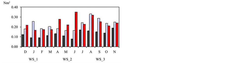
The seasonality of NE extreme wind stress in all points follows the seasonal pattern expected for the study area with peaks during spring (Figure 2). The average for spring season presents a value of 0.11 Nm⁻² on the oceanic region (ws_2, ws_3 and Q) and 0.07 Nm⁻² in coastal area (SPA and ws_1) with 74% in northeasterly. The ws_1 grid point, over the continent, has the lowest peaks in relation to other reanalysis points but the max-

imum values are observed in spring, with the highest value in November (0.19 Nm⁻²). The ws_2 point presents high peaks in spring and summer; August (0.33 Nm⁻²), September (0.29 Nm⁻²) and January (0.25 Nm⁻²). The ws_3 point presents the highest value in June (0.35 Nm⁻²), corresponding to the southwesterly, the other peaks are verified in April (0.28 Nm⁻²), August (0.32 Nm⁻²), spring and summer (Figure 2(a)). The ws_SPA point presents a peak in June (0.26 Nm⁻²), also corresponding to the southwesterly wind and in spring. The QuickSCAT (Q) point presents maximum values in March (0.42 Nm⁻²), June (0.37 Nm⁻²), August (0.41 Nm⁻²) and

September (0.44 Nm⁻²), all corresponding to the northeasterly winds (Figure 2(b)). The results obtained in the coastal area suggest the influence of the sea-breeze during the spring-summer as [34] . Sometimes when strong NE winds persist for several days, strong upwelling can develop with surface temperatures dropping near the coast, close to Cabo Frio [33] . The transport of BC follows the curve of annual variation of wind shear over the subtropical basin with a maximum during the summer and minimum during the winter [48] .

The curves for the pressure grid points show peaks between July and September (Figure 2(c)). It can be observed the relationship between the pressure and wind stress for the same months, referring to the pattern of the SASA that is a semi-stationary meteorological system, presenting a well emphasized seasonal movement. During the summer this system, over the continent, becomes weaker than winter, moving southerly and on its western side the winds blow northeasterly towards the southeastern coast of South America and they are more intense in the southeastern coast of Brazil [49] . This seasonal variability is one of the most important factors related to the occurrence of upwelling in the region of Arraial do Cabo, where the winds blow along the coastline from north to south push the surface waters offshore on spring-summer periods [11] .

The small number of occurrence of extreme southwesterly winds (Figure 3) verified in all points is associated with the number of frontal systems that reach the region, unlike of extreme northeasterly winds that presents higher percentage around 53% and 71% for ws_3 and SPA, respectively (Figure 3(a)). The predominance of NE winds indicates the seasonal variability of the SASA that leads upwelling in this region.

4.2. Extreme Seasonal Variability of the SST and Chemical and Biological Parameters

The seasonality of the extreme SST presents a well-defined pattern with maximum peaks from February to July, reaching the maxima value (24.5˚C) in April. The minimum peaks occur from September to January, reaching the minima value (15.9˚C) in November. It can be related to the presence of the phenomenon known as thermal inversion seasonal, which is typical on the region, when the TW and SACWS alternate, producing layers below the thermocline with higher temperatures in winter and lower ones in summer [50] . Another important aspect in seasonality of SST is the interaction of currents, such as wind-induced flows, near the continental shelf [51] related to the prevailing of the SASA with E-N winds blowing offshore the coastline and consequently leading to

occurrence of coastal upwelling. According to [52] the SST values are quite low from September to February and they start to increase gradually, reaching the maximum values in April.

Extreme seasonal variations were compared between SST, Chlorophyll a, Total Nitrogen (NO₂, NO₃, and NH₄), DO, PO₄, and peaks of larvae. DO presents maximum peak in February and June and two minimum peaks in April and July. Comparing the curves of DO with SST is verified values almost constant during spring and summer (Figure 4(a)). Total Nitrogen (Figure 4(b)) presents a small peak in February and another large one in September while phosphate presents a very sharp peak in September (Figure 4(c)). Chlorophyll a (Figure 4(d)) presents higher seasonal peak in February, being in accordance with DO. In this month occurs an increase of incidence of solar radiation with greater amount of nutrients and consequently increase of phytoplankton [53] . Smaller peaks are also observed in July, September and November. Studies commented by [54] affirm the existence of a negative correlation between Chlorophyll a and wind, in other words, when the wind is strong, primary production decreases. It can be explained due to the whitecapping breaking in the shallow water bodies lead to the production of short period waves under strong wind conditions that can prevent the transmission of light for phytoplankton [55] .

The maximum peaks of larvae are verified in November (Bryozoa, Isognomon, Mytilidae and Ostreidae), in December (Cypris) and in March (Bivalvia, Ascidiacea and Decapoda). These larvae as the other variables show a relationship with SST in the period of occurrence of upwelling with predominance of SACW in the region. However, Cirripedia and Polychaeta present peaks in July, they are found in warm and shallow waters (Figure 4(e)) In this month verifies the presence of the TW (warm) which at the western boundary is transported southward by the BC [56] . Cirripedia are sessile invertebrate organisms (barnacles) that cover substantial area of the substratum on intertidal and subtidal zones. They are important in determining and monitoring environmental impacts in coastal areas [57] . Although there are no further reports of economic damage, it is known that the hulls of ships, oil platforms, pipelines and other plant artificial substrates available in the marine environment may be completely covered by the barnacles causing corrosion of metals and an increase in maintenance costs [58] . The Polychaeta is a bristle-worm with species that live in the coldest ocean temperatures and other which tolerate the extreme high temperatures [59] .

4.3. Correlations between Physical, Chemical and Biological Variables

Measurement of joint range of variables is performed numerically by means of correlation coefficients that represent the degree of association between two continuous variables. The correlation is simply the tendency of the variables present their joint variation. Thus, the measure of correlation does not necessarily indicate that there is evidence of causal relationships between two variables. Evidence of causal relations must be obtained from the knowledge of the involved processes. The correlation coefficients calculated between extreme values of the physical and biological variables are presented in Table 3.

The results show small variability in spatial distributions of presented correlations. Correlations of the physical variables with nutrients and larvae present a relatively similar pattern for all points. These results suggest a

relationship with the extremes that occur in the upwelling process due to the positioning of SASA, sea level lowering and drop in SST. This leads to a linear relationship between them, showing that these variables have an interaction with the variations of sea level and temperature as well as the pressure and wind stress related to the meteorological forcing. The nutrients (PO₄, NO₂, NO₃ and NH₄), Chlorophyl a, DO and some larvae present positive (nutrients) and negative correlations (Table 3) with the wind stress points around 0.50. The maximumcorrelation is verified between NH₄ and ws_SPA (0.71).

The sea level lowering is in accordance with the increasing of nutrients and meroplankton larvae in the study area. The minimal meteorological residual presents a high correlation with NH₄ (−0.71), Bryosoa (−0.57) and NO₃ (−0.52), showing the influence by the SASA over the southeast coast of Brazil near Arraial do Cabo. These nutrients stimulates phytoplankton production, mainly larger species such as mesozooplankton and fisheries, being verified in several upwelling zones around the world such as in the SE Pacific Ocean, NE Pacific Ocean, NE Atlantic Ocean and Indian Ocean [10] .

These results are important on recovery as well as in monitoring environmental impacts in coastal regions and these larvae can be used as indicator organisms in monitoring programs due to their local distribution, lifestyle and tolerance to a large range of environmental conditions.

4.4. Multivariate Approaches

In PCA and factors analysis, the most commonly criteria used for solving the number of components is the eigenvalue criterion, for which only the components with eigenvalues greater than 1 are retained [60] .

In the present study, twenty-five variables were analyzed and six components were extracted with this criterion. Then the components that contain a greater variance than the original standardized variables are kept. The first component can be expected to have large amount of the total variance. Each succeeding component will account for progressively smaller amounts of variance. Therefore, only the first six components extracted have eigenvalues greater than 1 and account for 84.5% of the total variance in the dataset (Table 4). To maximize the variance of the first six principal axes, the Varimax normalized rotation was applied. The first three components are the most important and explain 25.1%, 18.8% and 12.9% of the variance, respectively (Table 4). Components 4 - 6 are not as important, and each of these three components explains a small amount of variance, between 10.2% and 8.1%. The first component explains the greatest amount of the variance, and is characterized by highly negative loadings in PA, PB and PSPA (Table 5). This statistical strategy gives greater importance to the pressure in the ordering and feature extraction of the spatial distribution. It suggests that the SASA plays a vital role in the Atlantic’s mean climatology. Variations in the position of the SASA are linked to seasonal variability of wind stress in the southeast coast of Brazil, leading to occurrence of upwelling. Because of this association, component 1 can be defined as the “pressure component” in reference to the main feature of the study area, associated with variations in the SASA pattern.

The second component is characterized by highly positively loadings in Total Nitrogen, Bryosoa and ws_1 (Table 5), and by highly negatively loadings in SST, being then mainly attributed to temperature, wind and nutrients related to local variables. These abiotic variables characterize a local marine ecosystem and are related to the presence of different water masses, being this component denominated “water masses component”, explaining the presence of SACW that is very important in upwelling periods.

The third component is characterized by positively loadings in Decapoda and Ascidiacea and by negatively loading in Cirripedia (Table 5). This component gives greater importance to the larvae and can be denominated “biotic component”, corresponding to the larvae economically important to the region as crustaceans. Cirripedia and Ascidiacea are a classes of zoobenthos and are found in intertidal zones. Ascidiaceas, for example, are larvae bioindicators that react to environmental changes with high filtration, playing a significant role in water purification. They influence the amount of nutrients and pollutants in suspension [61] [62] . But they grow rapidly and have a long reproduction period, becoming invasive potential, contributing to incrustation in the port regions [63] . Each of the last three components explains about 10.2%, 9.4% and 8.1% of variance, respectively and are clearly characterized by loadings in Salinity and DO (component 4), Bivalvia and Cypris (component 5) and Polychaeta (component 6) related to the marine conditions, indicating a physical and biological behavior for both components (Table 4).

The main result of the HCA performed on the 25 variables is the dendrogram (Figure 5). For this study, the Pearson-r distance was chosen as similarity measurement, between sampling sites. The sampling sites with the larger similarity are first grouped and next are joined with a linkage rule. The steps are repeated until all observations have been classified. Ward’s method was more successful to form clusters with the samples and are more or less homogenous, compared to other methods. Ward’s method is distinct from other linkage rules because it uses an analysis of variance approach to evaluate the distances between clusters [60] .

The classification of the samples into clusters is based on a visual observation of the dendrogram. The dendrogram shows two big clusters, one of most physical variables in one side and biological ones at the other, corresponding to the macrostructure of ecosystem (Figure 5). The degree of refinement of similarities can be expressed through a line that is drawn across the dendrogram at a linkage distance [64] . In this study, it was used a linkage distance of about 1.5 (Figure 5). Thus, samples with a linkage distance lower than 1.5 are grouped into several clusters. This line allows a division of the dendrogram into six clusters. Fewer or greater number of clusters could be defined by moving the position of the line up or down on the dendrogram. This subjective evaluation made HCA a semi-objective method.

Observation of the dendrogram reveals some indications of the level of similarity between the six clusters (Figure 5). Samples from cluster 1 (SST, residual, Cirripedia and Polychaeta), 2 (wind and nutrients) and 3

(pressure) are linked to the other clusters at an elevated distance, indicating that these samples are distinct from the ones of the other three clusters, i.e. cluster 4 (Salinity and DO), cluster 5 (Chlorophyll a, Decapoda, Ascidiacea, Bivalvia and Cypris) and cluster 6 (Mytilidae, Ostreidae, Bryozoa and Isognomon). It can thus be expected that the biological samples of cluster 5 would have similarities with the ones of cluster 6 because they are linked at a low distance.

The dendrogram is close to the PCA components, presenting clusters and loadings corresponding to six groups and factors, respectively, showing physical variables in one side and biological ones at the other.

5. Conclusions

Heterogeneous time series with weekly frequency shows seasonality and correlations between physical, chemical and biological variables in Arraial do Cabo as described in the literature. Reanalysis, QuikSCAT and surface station data show the strong influence of the SASA in the region. The data collected in the Anjos Bay, although weekly, show the characteristics of the aquatic environment in the studied period.

The wind stress at grid points 1, 2 and 3 as well as the pressure at A and B points (over the ocean) show higher peaks in spring months with predominance of northeasterly winds, characterizing the presence of the SASA.

The seasonality of minimum values of SST when compared to the Total Nitrogen, PO₄ and wind shows peaks in spring but when compared to the Chlorophyll a showsa very sharp peak in February. Maximum of larvae occur in November (Bryosoa, Isognomon, Mytilidae and Ostreidae), December (Cypris) and March (Bivalvia, Ascidiacea and Decapoda), months of upwelling. Maximum of Cirripedia and Polychaeta are found in July (down- welling period); they are found in warm (TW) and shallow waters and are important in determining and monitoring environmental impacts in coastal areas.

The correlations of the physical variables with nutrients and larvae present a relatively similar pattern for all points. These results suggest a relationship with the extremes that occur in the upwelling process due to the positioning of SASA, sea level lowering and SST reduction.

The first component of the PCA evidenced the influence of the SASA that is a major feature of the austral spring-summer climatology with the northeasterly winds that move surface waters offshore, leading a consequent upwelling of the SACW in Arraial do Cabo region. PCA shows that the highest variability is related to physical factors, nutrients, as well as larvae economically important to the coastal area of Arraial do Cabo city as crustaceans, mussels and oysters. The other components contribute with a small variance and are related to the biotic components of the classes of zoobenthos (Bivavia, Polychaeta and Cipris) found in intertidal zones, as well as DO and Salinity.

HCA grouped the samples in two big clusters with predominance of biotic variables in one side and abiotic ones at the other, corresponding to the macrostructure of ecosystem. In our study, the degree of refinement of similarities allowed a division into six clusters of samples, giving the most satisfactory results at forming distinct clusters (3, 4, 5 and 6) with more accurate regarding physical and biological elements.

Acknowledgements

The authors thank the Admiral Paulo Moreira Institute of Marine Studies-IEAPM of Brazilian Navy for data availability and logistical support. The authors also thank the collaboration of the Engineer Jose Maria de Castro Junior who provided logistical support for the acquisition of QuickSCAT data. Appreciation and thanks are given to the anonymous reviewer for the comments and suggestions to improve the manuscript. The authors also thank the financial support of the Coordination for the Improvement of Higher Level Personnel-Brazilian Research Agency (Capes).

Cite this paper

Marilia Mitidieri Fernandesde Oliveira,Gilberto CarvalhoPereira,Nelson Francisco FavillaEbecken,Jorge Luiz Fernandesde Oliveira, (2015) Multivariate Analysis of Extreme Physical, Biological and Chemical Patterns in the Dynamics of Aquatic Ecosystem. Journal of Environmental Protection,06,885-901. doi: 10.4236/jep.2015.68080

References

NOTES

^*Corresponding author.

References

- 1. Moore, T., Morris, K., Blackwell, G. and Gibson, S. (1997) Extraction of Beach Landforms from Dems Using a Coastal Management Expert System. Proceedings of Annual Conference of GeoComputation, Otago, 26-29 August 1997, 15-24.
- 2. Zalmon, I.R., Macedo, L.M., Rezende, C.E., Falcão, A.P.C. and Almeida, T.C. (2013) The Distribution of Macrofauna on the Inner Continental Shelf of Southeastern Brazil: The Major Influence of an Estuarine System. Estuarine Coastal Shelf Science, 130, 169-178.
http://dx.doi.org/10.1016/j.ecss.2013.03.001 - 3. Santos, I.R., Friedrich, A.C. and Ivar do Sul, J.A. (2009) Marine Debris Contamination along Undeveloped Tropical Beaches from Northeast Brazil. Environmental Monitoring Assessment, 148, 455-462.
http://dx.doi.org/10.1007/s10661-008-0175-z - 4. Salomon, A.K., Gaichas, S.K., Jensen, O.P., Agostini, V.N., Sloan, N.A., Rice, J., McClanahan, T.R., Ruckelshaus, M.H., Levin, P.S., Dulvy, N.K. and Babcock, E.A. (2011) Bridging the Divide between Fisheries and Marine Conservation Science. Bulletin of Marine Science, 87, 251-274.
http://dx.doi.org/10.5343/bms.2010.1089 - 5. Griffa, A., Lumpkin, R. and Veneziani, M. (2008) Cyclonic and Anticyclonic Motion in the Upper Ocean. Geophysical Research Letters, 35, Article ID: L01608, 1-5.
- 6. Myrberg, K., Andrejev, O. and Lehmann, A. (2010) Dynamic Features of Successive Upwelling Events in the Baltic Sea—A Numerical Case Study. Oceanologia, 52, 77-99.
http://dx.doi.org/10.5697/oc.55-3.687 - 7. Lorenzzetti, J.A., Wang, J.D. and Lee, T.N. (1987) Summer Upwelling on the Southeastern Continental Shelf of the USA during 1981. Progress in Oceanography, 19, 313-327.
http://dx.doi.org/10.1016/0079-6611(87)90010-3 - 8. Richter, I., Mechoso, C.R. and Robertson, W.A. (2008) What Determines the Position and Intensity of the South Atlantic Anticyclone in Austral Winter?—An AGCM Study. Journal of Climate, 21, 214-229.
http://dx.doi.org/10.1175/2007JCLI1802.1 - 9. Piontkovski, S.A., Landry, M.R., Finenko, Z.Z., Kovalev, A.V., Williams, R., Gallienne, C.P., Mishonov, A.V., Skryabin, V.A., Tokarev, Y.N. and Nikolsky, V.N. (2003) Plankton Communities of the South Atlantic Anticyclonic gyre: Communautés Planctoniques du Tourbillon Anticyclonique de l’Atlantique Sud. Oceanologica Acta, 26, 255-268.
http://dx.doi.org/10.1016/S0399-1784(03)00014-8 - 10. Guenther, M., Gonzalez-Rodrigues, E., Carvalho, W.F., Rezende, C.E., Mugrabe, G. and Valentin, J.L. (2008) Plankton Trophic Structure and Particulate Organic Carbon Production during a Coastal Downwelling-Upwelling Cycle. Marine Ecology Progress Series, 363, 109-119.
http://dx.doi.org/10.3354/meps07458 - 11. Pezzi, L.P. (2006) Variabilidade do Sistema Oceano-Atmosfera no Oceano Atlantico Sudoeste. I Seminário sobre sensoriamento remoto aplicado à pesca. INPE, São José dos Campos.
- 12. Castelao, R.M. and Barth, J.A. (2006) Upwelling around Cabo Frio, Brazil: The Importance of Wind Stress Curl. Geophysical Research Letters, 33, 1-4.
http://dx.doi.org/10.1029/2005gl025182 - 13. Calado, L., Gangopadhyay, A. and Da Silveira, I.C.A. (2008) Feature-Oriented Regional Modeling and Simulations (FORMS) for the Western South Atlantic: Southeastern Brazil Region. Ocean Modelling, 25, 48-64.
http://dx.doi.org/10.1016/j.ocemod.2008.06.007 - 14. Coelho-Souza, S.A., López, H.S., Guimarães, J.R.D., Coutinho, R. and Candella, N. (2012) Biophysical Interactions in the Cabo Frio Upwelling System, Southeastern Brazil. Brazilian Journal of Oceanography, 60, 353-365.
http://dx.doi.org/10.1590/S1679-87592012000300008 - 15. Valentin, J.L. and Coutinho, R. (1990) Modelling Maximum Chlorophyll in the Cabo Frio (Brazil) Upwelling: A Preliminary Approach. Ecological Modelling, 52, 103-113.
http://dx.doi.org/10.1016/0304-3800(90)90011-5 - 16. Topcu, D., Behrendt, H., Brockmann, U. and Claussen, U. (2010) Natural Background Concentrations of Nutrients in the German Bight Area (North Sea). Environmental Monitoring Assessment, 174, 361-388.
- 17. Morgan, R.P. and Kline, K.M. (2010) Nutrient Concentrations in Maryland Non-Tidal Streams. Environmental Monitoring Assessment, 178, 221-235.
http://dx.doi.org/10.1007/s10661-010-1684-0 - 18. Pereira, G.C., Figueredo, A.R., Jabor, P.M. and Ebecken, N.F.F. (2010) Assessing the Ecological Status of Plankton in Anjos Bay: A Flowcitometry Approach. Biogeoscience Discuss, 7, 6243-6264.
http://dx.doi.org/10.5194/bgd-7-6243-2010 - 19. Guimaraens, M.A. and Coutinho, R. (1996) Spatial and Temporal Variation of Benthic Marine Algae at the Cabo Frio Upwelling Region. Aquatic Botany, 52, 283-299.
http://dx.doi.org/10.1016/0304-3770(95)00511-0 - 20. Bakun, A. (1990) Global Climate Change and Intensification of Coastal Ocean Upwelling. Science, 247, 198-201.
http://dx.doi.org/10.1126/science.247.4939.198 - 21. Oliveira, M.M.F., de Pereira, G.C., Oliveira, J.L.F. and de Ebecken, N.F.F. (2012) Large and Mesoscale Meteo-Oceanographic Patterns in Local Responses of Biogeochemical Concentrations. Environmental Monitoring Assessment, 184, 6935-6953.
http://dx.doi.org/10.1007/s10661-011-2470-3 - 22. Oliveira, M.M.F., de Ebecken, N.F.F., Oliveira, J.L.F. and de Gilleland, E. (2011) Generalized Extreme Wind Speed Distributions in South America over the Atlantic Ocean Region. Theoretical Applied Climatology, 104, 377-385.
http://dx.doi.org/10.1007/s00704-010-0350-3 - 23. Kalnay, E. and Coauthors. (1996) The NCEP/NCAR 40 Year Reanalysis Project. American Meteorological Society, 177, 437-471. http://dx.doi.org/10.1175/1520-0477(1996)077<0437:TNYRP>2.0.CO;2
- 24. Vega, M., Pardo, R., Barrado, E. and Deban, L. (1998) Assessement of Seasonal and Polluting Effects on the Quality of River Water by Exploratory Data Analysis. Water Research, 32, 3581-3592.
http://dx.doi.org/10.1016/S0043-1354(98)00138-9 - 25. McArdle, B.H. and Anderson, M.J. (2001) Fitting Multivariate Models to Community Data: A Comment on Distance-Based Redundancy Analysis. Ecology, 82, 290-297.
http://dx.doi.org/10.1890/0012-9658(2001)082[0290:FMMTCD]2.0.CO;2 - 26. Reusch, T.B.H., Ehlers, A., Hämmerli, A. and Worm, B. (2005) Ecosystem Recovery after Climatic Extremes Enhanced by Genotypic Diversity. Proceedings of the National Academy of Sciences of the United States of America, 102, 2826-2831.
http://dx.doi.org/10.1073/pnas.0500008102 - 27. Silveira, I.C.A., Schimidt, A.C.K., Campos, E.J.D., Godoi, S.S. and Ikeda, Y. (2000) The Brazil Current off the Eastern Brazilian Coast. Brazilian Journal of Oceanography, 48, 171-183.
- 28. Soares, I. and Möller Jr., O. (2001) Low-Frequency Currents and Water Mass Spatial Distribution on the Southern Brazilian Shelf. Continental Shelf Research, 21, 1785-1814.
http://dx.doi.org/10.1016/S0278-4343(01)00024-3 - 29. Andrade, L., Gonzalez, A.M., Valentin, J.L. and Paranhos, R. (2004) Bacterial Abundance and Production in the Southwest Atlantic Ocean. Hydrobiology, 511, 103-111.
http://dx.doi.org/10.1023/B:HYDR.0000014033.81848.48 - 30. Campos, E.D., Miller, J.L., Muller, T.J. and Peterson, R.G. (1995) Physical Oceanography of the Southwest Atlantic Ocean. Oceanography, 8, 87-91.
http://dx.doi.org/10.5670/oceanog.1995.03 - 31. Pereira, G.C., Coutinho, R. and Ebecken, N.F.F. (2008) Data Mining for Environmental Analysis and Diagnostic: A Case Study of Upwelling Ecosystem of Arraial do Cabo. Brazilian Journal of Oceanography, 56, 1-18.
http://dx.doi.org/10.1590/S1679-87592008000100001 - 32. Valentin, J.L., Dalmo, A.L. and Salvador, J.A. (1987) Hydrobiology in the Cabo Frio (Brazil) Upwelling: Two-Dimensional Structure and Variability during Wind Cycle. Continental Shelf Research, 7, 77-88.
http://dx.doi.org/10.1016/0278-4343(87)90065-3 - 33. Valentin, J.L. (1984) Analyse des paramètres hydrobiologiques dans la remontée de Cabo Frio (Brésil). Marine Biology, 82, 259-276.
http://dx.doi.org/10.1007/BF00392407 - 34. Franchito, S.H., Rao, V.B., Stech, J.L. and Lorenzzetti, J.A. (1998) The Effect of Coastal Upwelling on the Sea-Breeze Circulation at Cabo Frio, Brazil: A Numerical Experiment. Annales Geophysicae, 16, 866-881.
http://dx.doi.org/10.1007/s00585-998-0866-3 - 35. Franchito, S.H., Rao, V.B., Oda, T.O. and Conforte, J. (2007) An Observational Study of the Evolution of the Atmospheric Boundary-Layer over Cabo Frio, Brazil. Annales Geophysicae, 25, 1735-1744.
http://dx.doi.org/10.5194/angeo-25-1735-2007 - 36. Ribeiro, F.N.D., Soares, J. and de Oliveira, A.P. (2011) The Co-Influence of the Sea-Breeze and the Coastal Upwelling at Cabo Frio: A Numerical Investigation Using Coupled Models. Brazilian Journal of Oceanography, 59, 131-144.
http://dx.doi.org/10.1590/S1679-87592011000200002 - 37. SCOR (1996) Protocols for the Joint Global Ocean Flux Study (JGOFS) Core Measurements. Scientific Committee on Ocean Research, International Council of Scientific Unions, Bergen, 170 p.
- 38. Richard, T.A. and Thompson, T.G. (1952) The Estimation and Characterization of Plankton Population by Pigment Analyses. A Spectrophotometric Method for the Estimation of Plankton Pigments. Journal of Marine Research, 11, 156-172.
- 39. Chao, Y., Li, Z., Kindle, J.C., Paduan, J.D. and Chavez, F.P. (2003) A High-Resolution Surface Vector Wind Product for Coastal Oceans: Blending Satellite Scatterometer Measurements with Regional Mesoscale Atmospheric Model Simulations. Geophysical Research Letters, 30, 13.1-13.4.
- 40. Tang, W., Liu, W.T. and Stiles, B.W. (2004) Evaluation of High-Resolution Ocean Surface Vector Winds Measured by QuikSCAT Scatterometer in Coastal Regions. IEEE Transactions on Geoscience Remote Sensing, 42, 1762-1769.
http://dx.doi.org/10.1109/TGRS.2004.831685 - 41. Atlas, R., Busalacchi, A.J., Ghil, M., Bloom, S. and Kalnay, E. (1987) Global Surface Wind and Flux Fields from Model Assimilation of Seasat Data. Journal of Geophysical Research, 92, 6477-6487.
http://dx.doi.org/10.1029/JC092iC06p06477 - 42. Stech, J.L. and Lorenzzetti, J.A. (1992) The Response of the South Brazil Bight to the Passage of Wintertime Cold Fronts. Journal of Geophysical Research, 97, 9507-9520.
http://dx.doi.org/10.1029/92JC00486 - 43. Anneville, O., Souissi, S., Gammeter, S. and Straile, D. (2004) Seasonal and Inter-Annual Scales of Variability in Phytoplankton Assemblages: Comparison of Phytoplankton Dynamics in Three Peri-Alpine Lakes over a Period of 28 Years. Freshwater Biology, 49, 98-115.
http://dx.doi.org/10.1046/j.1365-2426.2003.01167.x - 44. Sharma, S. (1996) Applied Multivariate Techniques. John Wiley and Sons Inc., New York, 512 p.
- 45. Abdi, H. and Williams, L.J. (2010) Principal Component Analysis, Wiley Interdisciplinary Reviews: Computation Statistics, 2, 387-515.
http://dx.doi.org/10.1002/wics.101 - 46. Bernardi, J.V.E., Lacerda, L.D., Dórea, J.G., Landim, P.M.B., Gomes, J.P.O., Almeida, R., Manzatto, A.G. and Bastos, W.R. (2009) Aplicação da Análise das Componentes Principais na ordenação dos parametros Físico-Quimicos no Alto Rio Madeira e Afluentes, Amazçãnia Ocidenta. Geochemical Brasilien, 23, 79-90.
http://www.geobrasiliensis.org.br/ojs/index.php/geobrasiliensis/article/viewFile/296/pdf - 47. Stewart, R.H. (2007) Introduction to Physical Oceanography. Texas A & M University, College Station, 353 pp.
- 48. Matano, R.P., Schlax, M. and Chelton, D.B. (2001) Seasonal Variability in the Southwestern Atlantic. Journal of Geophysical Research, 98, 18027-18035.
http://dx.doi.org/10.1029/93JC01602 - 49. Ahrens, C.D. (2000) Meteorology Today: An Introduction to Weather Climate and the Environment. 6th Edition, Brooks/ Cole, London.
- 50. De Mesquita, A.R. (1997) Marés, Circulação e Nível do mar na Costa Sudeste do Brasil.
http://www.mares.io.usp.br/sudeste/sudeste.html - 51. Stigebrandt, A. (1999) Resistance to Barotropic Tidal Flow in Straits by Baroclinic Wave Drag. Journal of Physical Oceanography, 29, 191-197.
http://dx.doi.org/10.1175/1520-0485(1999)029<0191:RTBTFI>2.0.CO;2 - 52. Franchito, S.H., Oda, T.O., Rao, V.B. and Kayano, M.T. (2008) Interaction between Coastal Upwelling and Local Winds at Cabo Frio, Brazil: An Observational Study. Journal of Applied Meteorology and Climatology, 47, 1590-1598.
http://dx.doi.org/10.1175/2007JAMC1660.1 - 53. Newell, R.I.E., Fisher, T.R., Holyoke, R.R. and Comwell, J.C. (2005) Influence of Eastern Oysters on Nitrogen and Phosphorus Regeneration in Chesapeake Bay, USA. NATO Science Series IV: Earth Environmental Science, 47, 93-120. http://dx.doi.org/10.1007/1-4020-3030-4_6
- 54. Neves, D.R.C.B., Pinho, J.L.S. and Vieira, J.M.P. (2008) Análise de Dados de Satélite Adequados à Caracterização da Produção Primária na Superfície Oceanica da Zee Portuguesa. Engenharia Civil-UM, 33, 125-138.
- 55. Jones, N.L. and Monismith, S.G. (2008) The Influence of Whitecapping Waves on the Vertical Structure of Turbulence in a Shallow Estuarine Embayment. Journal of Physical Oceanography, 38, 1563-1580.
http://dx.doi.org/10.1175/2007JPO3766.1 - 56. Oliveira, M.M.F., de Pereira, G.C., Oliveira, J.L.F. and de Ebecken, N.F.F. (2013) Effects of Sea Level Variation on Biological and Chemical Concentrations in a Coastal Upwelling Ecosystem. Journal of Environmental Protection, 4, 61-76.
http://dx.doi.org/10.4236/jep.2013.411A008 - 57. Apolinário, M. (2001) Variation of Populations Densities between Two Species of Barnacles (Cirripedia: Megabalaninae) at Guanabara Bay and Nearly Islands in Rio de Janeiro/RJ. Nauplius, 9, 21-30.
- 58. Champ, M.A. and Lowenstein, F.L. (1987) TBT—The Dilemma of High-Technology Antifouling Paints. Oceanus, 35, 69-77.
- 59. Rocha, M.B., Radashevsky, V. and Paiva, P.C. (2009) Espécies de Scolelepis (Polychaeta, Spionidae) de praias do Estado do Rio de Janeiro, Brasil. Biota Neotrópica, 9, 101-108.
http://dx.doi.org/10.1590/S1676-06032009000400012 - 60. Cloutier, V., Lefebvre, R., Terrien, R. and Savard, M.M. (2008) Multivariate Statistical Analysis of Geochemical Data as Indicative of the Hydrogeochemical Evolution of Groundwater in a Sedimentary Rock Aquifer System. Journal of Hydrology, 353, 294-313.
http://dx.doi.org/10.1016/j.jhydrol.2008.02.015 - 61. Narandio, S.A., Carvalho, J.L. and García-Gomes, J.C. (1996) Effects of Environmental Stress on Ascidians Populations in Algeciras Bay (Southerm Spain). Marine Ecology, 144, 119-131.
www.int-res.com/articles/meps/144/m144p119.pdf
http://dx.doi.org/10.3354/meps144119 - 62. Lambert, T.C.C. and Lambert, G. (1998) Non-Indigenous Ascidians in Southerm California Harbors and Marinas. Marine Biology, 130, 675-688.
http://dx.doi.org/10.1007/s002270050289 - 63. Bak, R.P.M., Joenje, M., De Jong, I., Lambrechts, D.Y.M. and Van Veghel, M.L.J. (1996) Long-Term Changes on Coral Reef in Booming Populations of a Competitive Colonial Ascidian. Marine Ecology, 133, 303-306.
www.int-res.com/articles/meps/133/m133p303.pdf
http://dx.doi.org/10.3354/meps133303 - 64. StatSoft Inc. (2004) STATISTICA (Data Analysis Software System), Version 7.