ABSTRACT

The appearance of a face is severely altered by illumination conditions that makes automatic face recognition a challenging task. In this paper we propose a Gaussian Mixture Models (GMM)-based human face identification technique built in the Fourier or frequency domain that is robust to illumination changes and does not require “illumination normalization” (removal of illumination effects) prior to application unlike many existing methods. The importance of the Fourier domain phase in human face identification is a well-established fact in signal processing. A maximum a posteriori (or, MAP) estimate based on the posterior likelihood is used to perform identification, achieving misclassification error rates as low as 2% on a database that contains images of 65 individuals under 21 different illumination conditions. Furthermore, a misclassification rate of 3.5% is observed on the Yale database with 10 people and 64 different illumination conditions. Both these sets of results are significantly better than those obtained from traditional PCA and LDA classifiers. Statistical analysis pertaining to model selection is also presented.

1. Introduction

Biometric Authentication denotes the technique of identifying people based on their unique physical (e.g. face, fingerprints, iris) or behavioral (e.g. gait, voiceprint) traits. The modern world has seen a rapid evolution of the technology of biometric authentication, prompted by an increasing urgency for security following the attacks of 9/11. They are used everywhere today from law enforcement to immigration to e-commerce transactions. Of all the biometrics in use today, facial biometrics are probably the most popular owing to the ease of capturing face images using non-intrusive means such as, surveillance equipment. The significance of face as a biometric is ever increasing today in various areas of homeland security as well. This includes the practice of recording biometric information (photo and fingerprint) of foreign passengers at all US airports (the US-VISIT program) and the proposed inclusion of digitized photos in passports. Of all biometrics, face is the most acceptable because it is the most common method used by humans in their visual interaction and perception. In fact, facial recognition is an important human ability—an infant innately responds to face shapes at birth and can discriminate his or her mother’s face from a stranger’s at the tender age of 45 hours ([1]). In addition, the method of acquiring face images is very simple and non-intrusive.

The growing importance of face recognition has led to much research in computer vision over the past few decades, with applications ranging from still, controlled mug-shot verification to dynamic face identification in a cluttered background. There are two different approaches to devising face identification systems: 1) feature-based; and 2) model-based. Feature-based methods make use of individualized facial characteristics such as distance between eyes, nose, mouth, and their shapes and sizes, as the matching criteria. Model-based systems use a statistical model to represent the pattern of some facial features (often the ones mentioned above), and some characteristics of the fitted model (parameter estimates, likelihood, etc.) are used as the matching criteria. Some well-known model-based approaches include Gaussian models ([2]), deformable models ([3]), and the inhomogeneous Gibbs models ([4]) that are particularly good at capturing the local details of a face using a minimax entropy principle. One class of flexible statistical models is Mixture Models ([5]). These models can represent complex distributions through an appropriate choice of its components to represent accurately the local areas of support of the true distribution. Apart from statistical applications, Gaussian Mixture Models (GMM), the most popular of the mixture models, have also been used in computer vision. For instance, [6] used GMM for modeling the shape and texture of face images.

The problem of human face identification under illumination variations is also well-researched ([7,8]). Illumination changes occur frequently in real face images and hence it is imperative to develop identification methods that are robust to these changes. [9] and [10] contain comprehensive surveys and reviews of current face recognition methods that work well under varying illumination conditions. [11] proposed an appearancebased algorithm for face recognition across pose by estimating the eigen light-field from a collection of images. [12] developed a bilinear model of an illumination subspace given arbitrary shape parameters from a 3D face model, while [13] devised a novel face recognition technique under variable lighting using harmonic Image Exemplars that employ only one training image. Although all these approaches to devising face recognition systems are based on the spatial domain pixel intensities, recently much research effort has focused on the frequency domain as well whose many useful properties have been successfully exploited in various signal processing applications ([14]). The frequency spectrum of an image consists of two components, the magnitude and phase. In 2D images particularly, the phase captures more of the image intelligibility than magnitude and hence is very significant for performing image reconstruction ([15]). [16] showed that correlation filters built in the frequency domain can be used for efficient face identification, and recently, [17] proposed correlation filters based only on the Fourier domain phase which perform as well as the original filters. [18] demonstrated that performing PCA in the frequency domain using only the phase spectrum outperforms spatial domain PCA and has attractive properties such as robustness to illumination variations. Furthermore, much work has also been done on face recognition based on the low-frequency DCT (Discrete Cosine Transform) coefficients ([19,20]). [21] also proposed a similar method which applied Genetic Algorithms to search appropriate weights to rescale low-frequency DCT coefficients. Besides the DCT, discrete wavelet transform (DWT) is another common method in face recognition. There are several similarities between the DCT and the DWT: 1) They both transform the data into frequency domain; 2) As data dimension reduction methods, they are both independent of training data compared to the PCA. Because of these similarities, there are also several studies on illumination invariant recognition based on the DWT ([22-24]). All these suggest that the frequency domain, particularly the phase spectra, has the potential of devising efficient identification methods. However, no work has been done, as per our knowledge, on developing model-based face identification systems in the frequency domain. Hence, in this paper we propose a novel GMM-based face identification system in the frequency domain exploiting the significance of the phase spectrum. Moreover, unlike many face recognition techniques that perform illumination normalization prior to classification ([19,25-27]), our method does not require it, and is able to perform training and testing using subsets of the original images. A preliminary version of this work appeared in [28].

The rest of the paper is organized as follows. Section 2 presents our proposed GMM approach for human identification. Section 3 provides a brief description of the two databases used in this work and presents the classification results along with a performance comparison with existing approaches. Finally, model selection methods are included in Section 4 and a discussion appears in Section 5.

2. Gaussian Mixture Models Based on Phase

Because of their ability to capture heterogeneity in a cluster analysis context, finite mixture models provide a flexible approach to the statistical modeling of a wide variety of random phenomena. As any continuous distribution can be approximated arbitrarily well by a finite mixture of normal densities, Gaussian mixture models (GMM) provide a suitable semiparametric framework for modeling unknown and complex distributional shapes. Mixtures can thus handle situations where a single parametric family fails to provide a satisfactory model for local variations in the observed data, and offer the scope of inference at the same time.

2.1. Background: Model and Parameter Estimation

Let be a random sample of size n where is a p-dimensional random vector with probability distribution f(y_j) on. Also, let θ denote the vector of the model parameters. We write a g-component mixture model in parametric form as:

(1)

where contains the unknown parameters. represents the model parameters for the

mixture component and is the vector of the mixing proportions with. When the mixture components have a multivariate Gaussian distribution, each component is given by:

(2)

(3)

where denotes the multivariate Gaussian density with mean vector and covariance matrix. Plugging (3) in (1), the mixture model has the form:

(4)

Among the methods used to estimate mixture distributions are graphical models, method of moments, maximum likelihood (based on EM) and Bayesian approaches using Markov Chain Monte Carlo (MCMC) methods. Although the application of MCMC methods is now popular, there are some difficulties that need to be addressed in the context of mixture models ([5]). Bayes estimators for mixture models are well-defined as long as the prior distributions are proper since improper priors yield improper posterior distributions. Another drawback is that when the number of components g is unknown, the parameter space is ill-defined, which prevents the use of classical testing procedures. But if a fixed g is used, this is not of any concern.

Although EM is the most popular estimation method for mixture models, we adopt the Bayesian estimation technique using a fixed g due to the following reasons. The Bayesian approach yields a nice framework for performing statistical inference based on the posterior distributions of the parameters which is not provided by the EM method. For instance, there are rigorous methods available to perform a systematic model selection for the Bayesian approach. [29] suggests that the EM-type approximation is not really an adequate substitute for the more refined numerical approximation provided by the Gibbs sampler. In particular, they show that EM is not as effective as the Gibbs sampler in estimating the marginal distributions for small datasets with few samples as is often the case with image-based data. More precisely, if the number of training samples is smaller than the number of estimable parameters, the Bayesian method creates no overflows in the estimation procedure. Moreover, [30] points out that EM is often slower to converge than the corresponding Gibbs sampler for Bayesian inference.

A key step in the Bayesian estimation method consists of the specification of suitable priors for all the unknown parameters in. This ensures that the posterior density will be proper, thereby allowing the application of MCMC methods to provide an accurate approximation to the Bayes solution. In particular, if we use conjugate priors, then the posterior distribution of can be written in a closed-form and computations are much simplified. The conjugate priors for mixtures of multivariate Gaussians are,

(5)

(The Wishart distribution is a multivariate generalization of the Gamma distribution). According to [31], the parameters of the prior distributions should be so chosen as to be fairly flat in the region where the likelihood is substantial and not much greater elsewhere, in order to ensure that the estimates are relatively insensitive to reasonable changes in the prior.

The posterior quantities of interest are approximated by the Gibbs sampler which allow the construction of an ergodic Markov chain with stationary distribution equal to the posterior distribution of. In particular, Gibbs sampling simulates directly from the conditional distribution of a subvector of given all the other parameters in and y (called the complete conditional). It yields a Markov chain

whose distribution converges to the true posterior distribution of the parameters. The point estimates of the parameters are formed by the posterior means, estimated by the average of the first N values of the Markov chain. To reduce error associated with the fact that the chain takes time to converge to the correct distribution, however, we discard the first samples as burn-in, usually chosen by visual inspection of plots of the components of the Markov chain which shows that the chain has “settled down” into its steady-state behavior. Thus our estimates are given by

(6)

2.2. Proposed Model Based on Phase Spectra

An experiment that illustrates the fact that phase captures more of the image intelligibility than magnitude is described in Hayes (1982) and is performed as follows. Let and denote two images. From these images, two other images and are synthesized as:

(7)

where denotes the inverse Fourier transform operation. What happens here is that captures the intelligibility of, while captures that of. This is shown in Figure 1, and we see

clearly that both the re-constructed images bear more resemblance to that original image to which the respective phase component belonged. This demonstrates the significance of phase in identifying a face.

Despite the well-established significance of phase in face identification, modeling the phase poses several difficulties. Perhaps the biggest challenge arises due to the fact that the phase is an angle and it lies between –π and π (Figure 2). Such a behavior is difficult to capture with the help of traditional statistical models based on stationarity assumptions. Besides, the phase angle is sensitive to distortions in images which means that it varies considerably across images of the same person under different lighting conditions. This calls for carefully choosing a suitable representation of phase for modeling purposes which we do in the following way: we divide the Fourier transform of an image by the magnitude at every frequency. The resulting images are of unit magnitude and we call them “phase-only’’ images. We then use the real and imaginary parts of these phase-only frequencies for modeling purposes, which are nothing but the sinusoids of the 2D Fourier transform (and). This is a simple and effective way of modeling phase, as it provides an adequate representation and at the same time does not suffer from any of the difficulties associated with direct phase angle modeling (such as constrained support). Moreover, exploratory studies show that there does not exist any significant amount of correlation among the sinusoids at the different frequencies (Figure 2), and hence it is reasonable to assume independence and model each frequency separately. This helps in reducing the complexity of the model considerably and simplifying computations. However, we note here that extension to the correlated case, although algebraically cumbersome, is straightforward.

Let and respectively denote the real and the imaginary part at the frequency of the phase spectrum of the image from the person, (the total number of frequencies in each direction for the images), (the total number of people in the dataset), (the total number of illumination levels in the dataset). We model each frequency separately and for each individual; that is, we

model where n denotes the total number of training images, as a mixture of bivariate normal distributions, the mixture components being given by

where

where and are respectively the frequency-wise means for the real and the imaginary parts, and the frequency-wise variances and is the correlation coefficient between the real and the imaginary parts. They form the unknown parameters of, so that. The mixture model for each frequency for each person can then be written as:

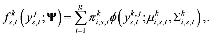(8)

where. It is a commonly known fact in signal processing that an image of good quality and identifiability can reconstructed using only few low frequency components around the origin ([14]). So we model only the low frequencies within a square grid region (determined by experimentation so that p is much smaller than M) around the origin of the spectral plane. Moreover, owing to the Hermitian symmetry of the frequency components, only half of these frequencies need to used in the model (real part is symmetric and imaginary part is anti-symmetric). The complete model for each person is then given by (based on the independence assumption):

(9)

The mixture components are expected to represent the different illumination levels in the images of each person.

2.3. Classification Scheme

We use a MAP (maximum a posteriori) estimate based on the posterior likelihood to classify the test images. For a new observation extracted from the phase spectrum of a test image, we can compute the likelihood under the model for person by evaluating

(10)

where is as in Equation (9). The posterior likelihood of the observed data belonging to a specific person is then be given by:

(11)

where denotes the prior probability for each person which we assume to be uniform over all the possible people in the database. A particular image will then be assigned to class if:

(12)

For computational convenience, it is a convention to work with log-likelihoods in order to avoid numerical overflows/underflows in the evaluation of Equation (10).

3. Results

In this section, we present the results of human classification. But first we briefly describe the two datasets used to illustrate the proposed techniques in this paper.

3.1. Face Image Datasets

First, we use a subset of the publicly available “CMUPIE Database” ([32]) which contains images of people captured under different illumination conditions ranging from shadows to balanced and overall dark. Figure 3 shows a small sample of images of 6 people under 3 different lighting effects.

All these images are cropped using affine transformations based on locations of the eyes and nose as is common and necessary for most computer vision problems ([33]) for a detailed overview of such a cropping technique). The final cropped images are of dimension 100 × 100.

The second database is a susbset of the “Yale Face Database B” ([7]), consisting of images of 10 individuals under 64 different illumination conditions. Some sample images are shown in Figure 4. These images are again cropped and aligned in a similar manner as the PIE images, and the final images are of dimension 90 × 80.

Note here that for both these sets, we use only frontal

images under varying lighting conditions since our objective is to study the illumination problem in this paper.

3.2. Classification Results

For both the datasets, we select M = 50 and this succeeds in reducing the dimensionality of the problem considerably (from 100 × 100 = 10000 frequencies to 50 × 25 = 1250 frequencies for the PIE images and from 90 × 80 = 7200 frequencies to 1250 frequencies for the Yale images). Recall that there are J = 21 illumination levels in the images of a person in the CMU-PIE database, and J = 64 in the images of a person in the Yale database.

We start with g = 2 and use a total of N = 5000 iterations of the Gibbs sampler allowing a burn-in of for each frequency. We select different training and test sets for each person to study how the number of training images affect the classification results. The training images in each case are randomly selected and the rest used for testing. Furthermore, this selection of training set is repeated 20 times (in order to remove selection bias) and the final errors are obtained by averaging over the 20 iterations. Tables 1 and 2 summarize the classification results from applying our classification method to the two datasets. The tables also include the standard deviations of the corresponding error rates over the 20 repetitions, as measures of reliability of the quantities.

The results on the two databases illustrate that our proposed method is quite effective in dealing with a large number of individuals (PIE database) as well as a large number of illumination conditions (Yale database). This is particularly impressive given the fact that no illumination normalization is performed prior to classification, and both training and testing are done on the original cropped images with varying illumination. This demonstrates that the statistical model used is able to aptly capture the discriminative facial details of each person

despite the distortions caused by non-uniform lighting. The classification results deteriorate as the size of the training set decreases. This is expected since an adequate number of training images is required for the efficient estimation of all the model parameters. The training set in each case is selected randomly, hence the classification performance does not depend on the nature of the training images selected. Furthermore, the associated standard deviations over the repetitions in each case is quite low, thus demonstrating that the results are not sensitive to training set selection. Our method thus appears to be robust to widely varying training and test sets and this suggests that the representation of phase in our model succeeds in forming a valid human identification system.

3.3. Performance Comparison

We now conduct a comparative study of the identification performance of our GMM-based method with those from some existing methods applied to the same subsets of the two database. The competing classifiers used are Principal Components Analysis (PCA) and Linear Discriminant Analysis (LDA), the results being included in Table 3. For the PIE database, we use the results with g = 2 and 10 training images, and for Yale, we use g = 3 and 20 training images.

As we can see clearly, both the traditional PCA and LDA classifiers fail completely for both datasets, yielding high misclassification error rates, and our proposed GMM-based method outperforms them by an overwhelming margin.This is because both these traditional methods are very sensitive to illumination variations and thus perform poorly. We cannot compare our method to that in Gross, Matthews and Baker (2004) since they used a different subset of the CMU-PIE database that has different poses for a single person. Our current model was developed to be robust to illumination changes and hence only frontal images were used. However, we wish to extend this model to apply to images with multiple poses as well, as we discuss later on in the paper. Most face identification methods that are in use today use illumination normalization methods to first eliminate the illumination variations in the image and then apply the classifier on the restored or normalized images that are free from such variations ([19,25,26,34]). In contrast, our proposed approach does not require removing the illumination variations from the images prior to classification,

a significant improvement over existing methods.

4. Choosing the Number of Mixture Components

Often we can improve model fit and classification accuracy by using a greater number of mixture components. Recall that, in our models, the mixtures represent the different illumination conditions in the images of a person. It is therefore reasonable to expect that the number of components should depend directly on the nature of illumination variation among the training images. For example, for a small set, say with 3 or 6 images, there is insufficient data to be able to display much variation, and at the same time estimate effectively all the additional parameters associated with a larger g. Thus, increasing the number of mixture components when using few training images is not worthwhile. However, increasing the number of mixture components may be beneficial to classification performance when a sufficiently large training set is used. With more images, it is likely that the images will vary significantly with respect to the nature of illumination, and this may be better captured with more mixture components in the form of efficient clustering.

We use and with cases 1) and 2) for both datasets. The results are included in Table 4, along with the standard deviations computed over different training sets. The results for the PIE database are not significantly better than those from using g = 2 (p-values > 0.9 in all cases). We thus conclude that g = 2 is the optimal choice for this particular database as far as the trade-off between model complexity and classification performance is concerned. For the Yale database, on the other hand, we observe significant improvements in the classification performance for both the cases with g = 3 (p-value < 0.001). However, significant improvement is limited when the number of mixture components was further increased to g = 4 (p-value > 0.4). Therefore, g = 3 can be taken to be optimal for this dataset. We see similar results when applying Bayes factors ([35]) to perform model selectionthe model with g = 2 components is preferred for the PIE databases whereas the model with g = 3 has significantly better performance for the Yale database. These results can be explained by the fact that the images in the Yale database has more varying illumination levels than those in the PIE database (64 different illumination conditions for Yale and for PIE), hence a larger number of mixture components are required to model that.

We note here that a GMM with g = 1 (the traditional bivariate Gaussian model with no mixture components) performed really poorly in all cases, yielding misclassification rates of over 50%. This shows that a single Gaussian distribution is unable to capture the inherent variability present in the different images due to illumination effects that are aptly captured by the GMMs.

5. Discussion

In this paper, we have introduced a novel face identification scheme based on phase and GMMs. Although the importance of phase is well-known, this fact had not yet been utilized in building model-based identification techniques. This is partially because modeling phase with the help of an appropriate representation of its variability across different images of a person is indeed a challenging task and our experiments show that our proposed models are able to handle it fairly well. We point out again that the novelty of our method lies in the fact that the human identification method does not need to rely on removing the lighting effects in advance like many existing work, and works directly on the raw images with extreme illumination variations. Not only this, we have demonstrated that our approach is tolerant to illuminations; in fact, the model has a general framework and we are exploring applications of our methodology to images with expression and pose variations. Thus this should be useful in practice for handling real life databases that are often subject to extraneous variations. Very good identification error rates of about 2% are obtained. In conclusion, both GMM and phase have enormous potential in computer vision, and harnessing this combined strength has indeed proved to be a success.

So far we have seen that research on face recognition has been primarily limited within the computer science community although statistical and probabilistic models are used widely in developing such identification tools. For instance, in this paper we have established the utility of the well-known statistical technique of mixture models (GMMs actually) in building efficient face recognition techniques. The low misclassification error rates from

our classifier show that it helps achieve this goal successfully. Our immediate future direction of work consists of assessing the performance of our GMM model on larger and more diverse databases with expression and pose variations. For both the latter types of variations, we would expect the mixture components to represent their various levels; for instance, for images with 3 different expressions (say, happy, sad, disgust), we would use a GMM with g = 3 components.

6. Acknowledgements

The authors’ research was supported in part by a research grant from the Army Research Office (ARO) to CyLab, Carnegie Mellon. The author would like to thank Dr. Stephen Fienberg, Dr. Anthony Brockwell of Carnegie Mellon University for various helpful suggestions during the course of this research work and Dr. Marios Savvides and Dr. Yanxi Liu, CMU, for the databases used for this work.

REFERENCES

- D. Voth, “In the News: Face Recognition Technology,” IEEE Magazine on Intelligent Systems, Vol. 18, No. 3, 2003, pp. 4-7.
- M. A. Turk and A. P. Pentland, “Face Recognition Using Eigenfaces,” Proceedings of IEEE Conference on Computer Vision and Pattern Recognition, Maui, 3-6 June 1991, pp. 586-591.
- A. Yuille, “Deformable Templates for Face Recognition,” Journal of Cognitive Neuroscience, Vol. 3, No. 1, 1991, pp. 59-70. doi:10.1162/jocn.1991.3.1.59
- C. Liu, S. C. Zhu and H. Y. Shum, “Learning Inhomogeneous Gibbs Model of Faces by Minimax Entropy,” IEEE International Conference on Computer Vision, Vancouver, July 2001, pp. 281-287.
- G. McLachlan and D. Peel, “Finite Mixture Models,” John Wiley and Sons, Hoboken, 2000. doi:10.1002/0471721182
- S. Zhu, Y. Wu and D. Mumford, “Minimax Entropy Principle and Its Application to Texture Modeling,” Neural Computation, Vol. 9, No. 8, 1997, pp. 1627-1660. doi:10.1162/neco.1997.9.8.1627
- A. S. Georghiades, P. N. Belhumeur and D. J. Kreigman, “From Few to Many: Illumination Cone Models for Face Recognition under Variable Lighting and Pose,” IEEE Transactions on Pattern Analysis and Machine Intelligence, Vol. 23, No. 6, 2001, pp. 643-660. doi:10.1109/34.927464
- K. Lee, J. Ho and D. Kreigman, “Nine Points of Light: Acquiring Subspaces for Face Recognition under Variable Lighting,” IEEE Conference on Computer Vision and Pattern Recognition, Vol. 1, 2001, pp. 519-526.
- Z. Lian and M. Joo Er, “Face Recognition under Varying Illumination,” New Trends in Technologies: Control, Management, Computational Intelligence and Network Systems, 2010, pp. 209-226. doi:10.5772/10413
- X. Zou, J. Kittler and K. Messer, “Illumination Invariant Face Recognition: A Survey,” Proceedings of the First IEEE International Conference on Biometrics: Theory, Applications and Systems, Washington DC, September 2007, pp. 1-8.
- R. Gross, I. Matthews and S. Baker, “Appearance Based Face Recognition and Light-Fields,” IEEE Transactions on Pattern Analysis and Machine Intelligence, Vol. 26, No. 4, 2004, pp. 449-465. doi:10.1109/TPAMI.2004.1265861
- J. Lee, B. Moghaddam, H. Pfister and R. Machiraju, “A Bilinear Illumination Model for Robust Face Recognition,” IEEE International Conference on Computer Vision, Vol. 2, 2005, pp. 1177-1184.
- L. Zhang and D. Samaras, “Face Recognition under Variable Lighting Using Harmonic Image Exemplars,” IEEE Conference on Computer Vision and Pattern Recognition, Vol. 1, 2003, pp. 19-25.
- A. V. Oppenheim and R. W. Schafer, “Discrete-Time Signal Processing,” Prentice Hall, 1989.
- M. H. Hayes, “The Reconstruction of a Multidimensional Sequence from the Phase or Magnitude of Its Fourier Transform,” IEEE Transactions on Acoustics, Speech and Signal Processing, Vol. 30, No. 2, 1982, pp. 140-154. doi:10.1109/TASSP.1982.1163863
- M. Savvides, B. V. K. Vijaya Kumar and P. Khosla, “Face Verification Using Correlation Filters,” 3rd IEEE Automatic Identification Advanced Technologies, Tarrytown, 2002, pp. 56-61.
- M. Savvides and B. V. K. Vijaya Kumar, “Eigenphases vs. Eigenfaces,” Proceedings of International Conference on Pattern Recognition, Vol. 3, 2004, pp. 810-813.
- M. Savvides, B. V. K. Vijaya Kumar and P. K. Khosla, “Corefaces—Robust Shift Invariant PCA Based Correlation Filter for Illumination Tolerant Face Recognition,” Proceedings of IEEE Conference on Computer Vision and Pattern Recognition, Vol. 2, 2004, pp. 834-841.
- W. Chen, M. J. Er and S. Wu, “Illumination Compensation and Normalization for Robust Face Recognition Using Discrete Cosine Transform in Logarithm Domain,” IEEE Transactions on Systems, Man and Cybernetics, Vol. 36, No. 2, 2006, pp. 458-466. doi:10.1109/TSMCB.2005.857353
- V. P. Vishwakarma, S. Pandey and M. N. Gupta, “A Novel Approach for Face Recognition Using DCT Coefficients Re-Scaling for Illumination Normalization,” International Conference on Advanced Computing and Communications, Guwahati, 18-21 December 2007, pp. 535-539.
- C. A. Perez and L. E. Castillo, “Genetic Improvements in Illumination Compensation by the Discrete Cosine Transform and Local Normalization for Face Recognition,” The International Society for Optical Engineering, International Symposium on Optomechatronic Technologies, Vol. 7266, 2008, pp. 1-8.
- X. F. Nie, Z. F. Tan and J. Guo, “Face Illumination Compensation Based on Wavelet Transform,” Optics and Precision Engineering, Vol. 16, No. 1, 2008, pp. 971-987.
- H. Han, S. G. Shan, X. L. Chen and W. Gao, “Illumination Transfer Using Homomorphic Wavelet Filtering and Its Application to Light-Insensitive Face Recognition,” International Conference on Automatic Face and Gesture Recognition, Amsterdam, 17-19 September 2008, pp. 1-6. doi:10.1109/AFGR.2008.4813380
- W. G. Gong, L. P. Yang, X. H. Gu and W. H. Li, “Illumination Compensation Based on Multi-Level Wavelet Decomposition for Face Recognition,” Optics and Precision Engineering, Vol. 16, No. 8, 2008, pp. 1459-1464.
- T. Chen, W. Yin, X. S. Zhou, D. Comaniciu and T. S. Huang, “Illumination Normalization for Face Recognition and Uneven Background Correction Using Total Variation Based Image Models,” IEEE Conference on Computer Vision and Pattern Recognition, Vol. 2, 2005, pp. 532-539.
- D. H. Liu, L. S. Shen and K. M. Lam, “Illumination Invariant Face Recognition,” Pattern Recognition, Vol. 38, No. 10, 2005, pp. 1705-1716. doi:10.1016/j.patcog.2005.03.009
- X. Xie and K. M. Lam, “Face Recognition under Varying Illumination Based on a 2D Face Shape Model,” Pattern Recognition, Vol. 38, No. 2, 2005, pp. 221-230. doi:10.1016/j.patcog.2004.07.002
- S. Mitra and M. Savvides, “Gaussian Mixture Models Based on Phase Spectra for Human Identification and Illumination Classification,” Proceedings of 14th IEEE Workshop on Automatic Identification Advanced Technologies, Buffalo, October 2005.
- A. E. Gelfand, S. E. Hills, A. Racine-Poon and A. F. M. Smith, “Illustration of Bayesian Inference in Normal Data Models Using Gibbs Sampling,” Journal of the American Statistical Association, Vol. 85, No. 412, 1990, pp. 972- 985. doi:10.1080/01621459.1990.10474968
- S. K. Sahu and G. O. Roberts, “On Convergence of the EM Algorithm and the Gibbs Sampler,” Statistics and Computing, Vol. 9, No. 1, 1999, pp. 55-64. doi:10.1023/A:1008814227332
- H. Bensmail, G. Celeux, A. Raftery and C. P. Robert, “Inference in Model-Based Cluster Analysis,” Statistics and Computing, Vol. 7, No. 1, 1997, pp. 1-10. doi:10.1023/A:1018510926151
- T. Sim, S. Baker and M. Bsat, “The CMU Pose, Illumination, and Expression (PIE) Database,” Proceedings of the 5th International Conference on Automatic Face and Gesture Recognition, Washington DC, 20-21 May 2002, pp. 46-51. doi:10.1109/AFGR.2002.1004130
- Y. Liu, K. Schmidt, J. Cohn and S. Mitra, “Facial Asymmetry Quantification for Expression-Invariant Human Identification,” Computer Vision and Image Understanding, Vol. 91, No. 1-2, 2003, pp. 138-159. doi:10.1016/S1077-3142(03)00078-X
- H. Wang, S. Z. Li and Y. Wang, “Face Recognition under Varying Lighting Conditions Using Self Quotient Image,” IEEE Conference on Automatic Face and Gesture Recognition, 17-19 May 2004, pp. 819-824. doi:10.1109/AFGR.2004.1301635
- R. E. Kass and A. E. Raftery, “Bayes Factors,” Journal of the American Statistical Association, Vol. 90, No. 430, 1995, pp. 773-795. doi:10.1080/01621459.1995.10476572