ABSTRACT

The concept of normal form is used to study the dynamics of non-linear systems. In this work we describe the normal form for vector fields on with linear nilpotent part made up of coupled n Jordan blocks. We use an algorithm based on the notion of transvectants from classical invariant theory known as boosting to equivariants in determining the normal form when the Stanley decomposition for the ring of invariants is known.

1. Introduction

There are well-known procedures for putting a system of differential equations (where v is a formal power series starting with quadratic terms) into normal form with respect to its linear part A. Our concern in this paper is to describe the normal form of the systemm, that is the set of all v such that is in normal form where A is the linear part from the Stanley decomposition of the ring of invariants. Our main result is a procedure that solves the description problem where N is a nilpotent matrix with coupled n Jordan blocks, provided that the description problem is already solved for each Jordan block of N taken separately. Our method is based on adding one block at a time. This procedure will be illustrated with examples and then be generalized.

The idea of simplification near an equilibrium goes back at least to Poincare (1880), who was among the first to bring forth the theory in a more definite form. Poincare considered the problem of reducing a system of nonlinear differential equations to a system of linear ones. The formal solution of this problem entails finding nearidentity coordinate transformations, which eliminate the analytic expressions of the nonlinear terms.

Cushman et al. [1], using a method called covariant of special equivariant solved the problem of finding Stanley decomposition of. Their method begins by creating a scalar problem that is larger than the vector problem and their procedures are derived from classical invariant theory thus it was necessary to repeat calculations of classical invariants theory at the levels of equivariants. Malonza [2] solved the same problem by “Groebner” basis methods found in [3] rather than borrowing from classical theory.

Murdock and Sanders [4] developed an algorithm based on the notion of transventants to determine the form of normal form of a vector field with nilpotent linear part, when the normal form is known for each Jordan block of the linear part taken separately. The algorithm is based on the notion of transvectants from the classical invariant theory known as boosting to module of equivariants when the Stanley decomposition for the ring of invariants is known.

Namachchivaya et al. [5], studied a generalized Hopf bifurcation with non-semisimple 1:1 Resonance. The normal form for such a system contains only terms that belong to both the semisimple part of A and the normal form of the nilpotent, which is a coupled TakensBogdanov system with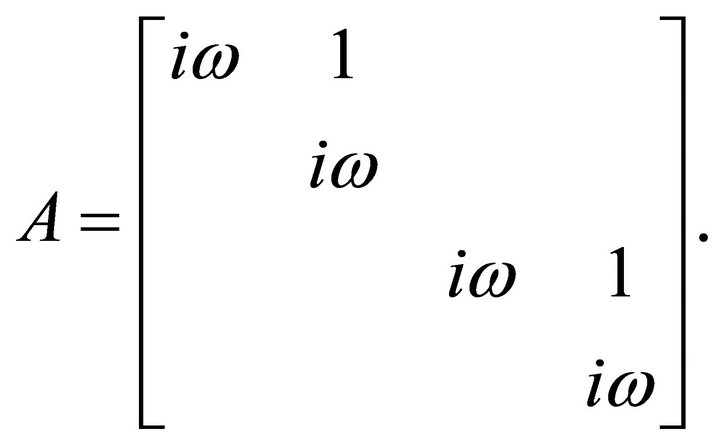

This example illustrates the physical significance of the study of normal forms for systems with nilpotent linear part.

Our results are mainly based on the work found in [4] that is application of transvectant’s method for computing normal form for the module of equivariants of nilpotent systems. In section two and three we put together background knowledge for understanding the content of this work. Section four forms the central part of this paper where we shall compute the module of equivariants.

2. Invariants and Stanley Decompositions

Let denote the vector space of homogeneous polynomials of degree on with coefficients in, where denotes the set of real numbers. Let be the vector space of all such polynomials of any degree and let be the vector space of formal power series. If, becomes the ring of formal power series on, where denotes the set of real numbers. For such smooth vectors fields, it is sufficient to work polynomials. For any nilpotent matrix, we define the Lie operator

by

(2.1)

and the differential operator

by

(2.2)

Then is a derivation of the ring, meaning that

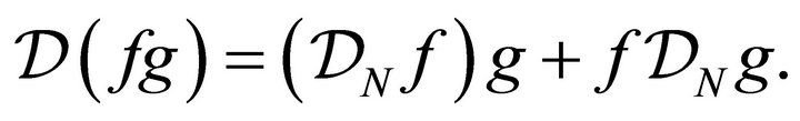(2.3)

In addition,

(2.4)

A function is called an invariant of if

or equivalently Since

it follows that if f and are invariants, so are amd; that is is both a vector space over and also a subring of, known as the ring of invariants. Similarly a vector field is called an equivariants of, if that is

There are two normal form styles in common use for nilpotent systems, the inner product normal form and the sl(2) normal form. The inner product normal form is defined by where is the conjugate transpose of. To define the sl(2) normal form, one first sets and constructs matrices and such that

(2.5)

An example of such an triad is

Having obtained the triad we create two additional triads and as follows

(2.6)

(2.7)

The first of these is a triad of differential operators and the second is a triad of Lie operators. Both the operators and inherit the triad properties (2.5). Observe that the operators map each

into itself. It follows from the representation theory that

(2.8)

Clearly the ia s subring of, the ring of invariants and it follows from (2.4) that is a module over this subring. This is the sl(2) normal form module.

3. Boosting Rings of Invariants to Module of Equivariants

In this section we describe the procedure for obtaining a Stanley decomposition of the module of equivariants (or normal form space) when the Stanley decomposition of the ring of invariants is known.

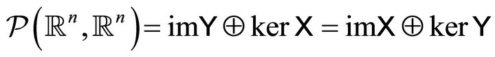
The module of all formal power series vector fields on can be viewed as the tensor product , and in fact the tensor product can be identified with the ordinary product (of a field times a constant vector) since the ordinary product satisfies the same algebraic rules as a tensor product. Specifically, every formal power series vector field can be written as

where the are the standard basis vectors of. Next, the Lie derivative can be expressed as the tensor product of and, that is . Under the identification of with ordinary product, this means

, where

and in agreement with the following calculation, in which because is constant.

This kind of calculation also shows that representation (on vector fields ) with triad is the tensor product of the representation (on scalar fields)

with triad and the representation (on

with triad that is

It follows that a basis from the normal form space is given by well defined transvectants

as ranges over a basis for

and ranges over a basis for. The first of these bases is given by the standard monomials of a Stanley decomposition for. The second is given by the standard basis vectors such that is the index of the bottom row of a Jordan block in. It is useful to note that the weight of such an is one less than the size of the block. Then we define the transvectant as

From here, the computational procedures of box products are the same as those used in describing rings of invariants from [4], except that infinite iterations never arise.

4. Normal Form for Systems with Linear Part N_3(n)

Before generalizing we shall consider the normal form for nonlinear systems with linear part having two and three blocks, that is and as examples.

4.1. System with Linear Part N₃₃

The Stanley decomposition for the ring of invariants with linear part is given by:

(see [6]). Since and has weight zero, it is convenient to remove them since we do not expand along terms of weight zero by setting and write

In this case the basis elements are and. Therefore we need to compute the box product of the ring with which are both of weight 2.

Therefore. Distributing the box product there are two cases to consider.

Case 1:

.

There are four products namely:

a)

b)

c)

d)

Recombining terms gives

Case 2: Similarly we have,

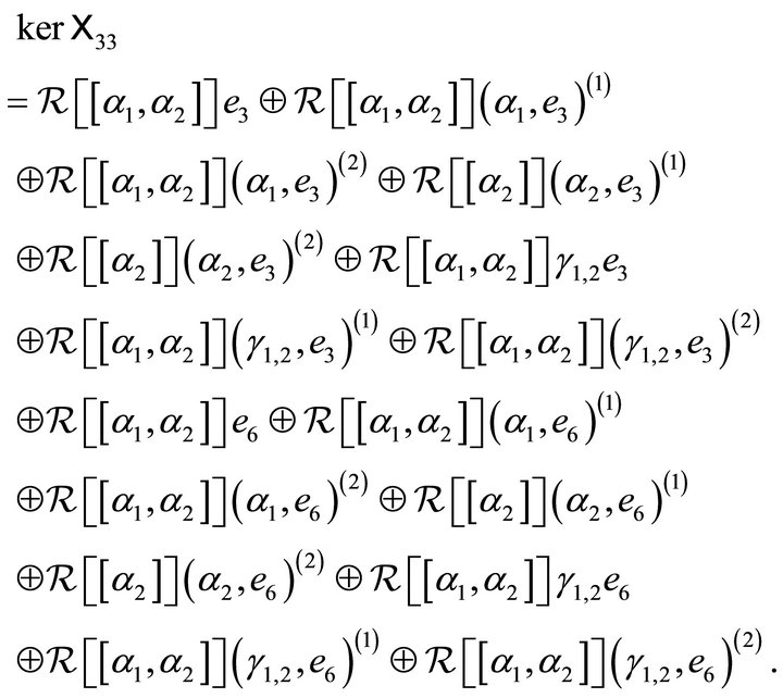
Adding terms in case 1 and 2 we obtain:

Finally, to complete the calculation, it is necessary to compute the transvectants that appear. These are of the form and for where.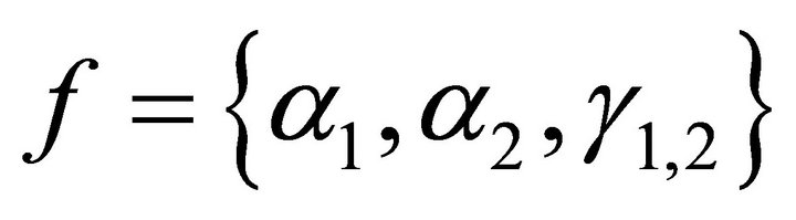

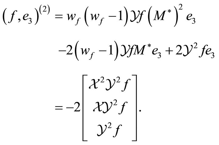
We ignore the nonzero constants –1 and –2 because we are concerned with computing basis elements. For the basis we have:

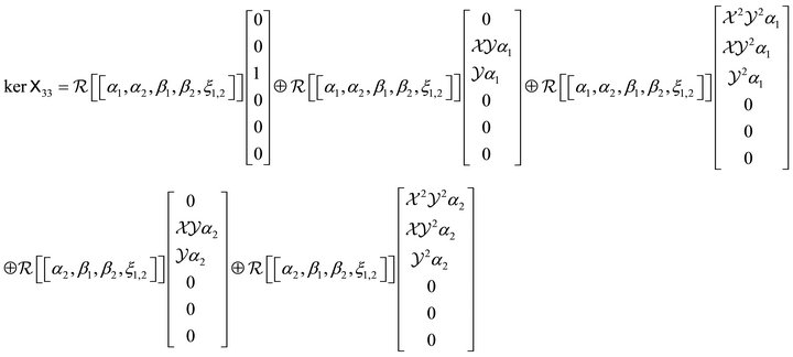
Therefore the normal form for system with linear part is:

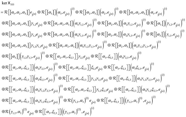
4.2. System with Linear Part N₃₃₃

The Stanley decomposition for ring of invariants of a system with linear part is given by:

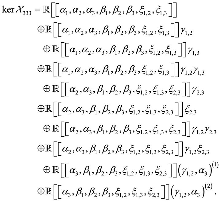
(see [6]).

The basis elements for are and. Therefore we need to compute the box product of the invariants ring with. Thus Let

, then

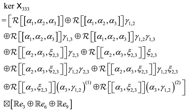
There are three cases to consider. Computing and simplifying the cases we obtain the normal form as:

where and such that,

and

In general, from the above examples we conclude that the normal forms are obtained by computing the box product

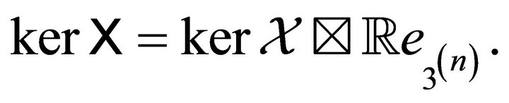
The basis of the normal form of are transvectants of the form: where is the standard monomials of Stanley decomposition of the ring of invariants, , and.

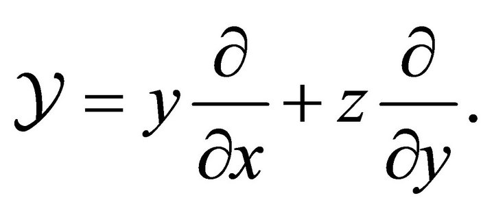
As an example we find the normal form for a system with linear part, we first find the ring of invariants

where using. By inspection and, and this generates the entire ring; that is

(4.1)

To check this, we note that the weight of is two and is of weight zero, so the table function of is

Hence

this implies (0.1).

The next step is to compute as a module over. contains one Jordan block of size 3 hence the differential operators

In this case the basis elements is which is of weight 2 therefore the normal form is

We compute:

The differential equations in normal form are:

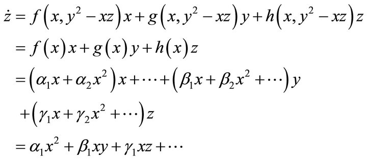
The normal form upto quadratic term is:

Remark: The normal form of a dynamical systems is a powerful tool in the study of stability and bifurcations analysis. From the practical point of view, only the normal form with perturbation (bifurcation) parameters is useful in analyzing physical or engineering problems. In this paper the computation of the normal form has been mainly restricted to systems which do not contain perturbation parameters by setting the parameters to zero to obtain the simplified normal form. Having found the normal form of the reduced system we shall then add unfolding terms to get a parametric normal form for bifurcation analysis.

REFERENCES

NOTES

^*Corresponding author.

REFERENCES

- R. Cushman, J. A. Sanders and N. White, “Normal Form for the (2;n)-Nilpotent Vector Field Using Invariant Theory,” Physica D: Nonlinear Phenomena, Vol. 30, No. 3, 1988, pp. 399-412. doi:10.1016/0167-2789(88)90028-0
- D. M. Malonza “Normal Forms for Coupled Takens-Bogdanov Systems,” Journal of Nonlinear Mathematical Physics, Vol. 11, No. 3, 2004, pp. 376-398. doi:10.2991/jnmp.2004.11.3.8
- W. W. Adams and P. Loustaunau, “An Introduction to Gröbner Bases,” American Mathematical Society, Providence, 1994.
- J. Murdock and J. A. Sanders, “A New Transvectant Algorithm for Nilpotent Normal Forms,” Journal of Differential Equations, Vol. 238, No. 1, 2007, pp. 234-256. doi:10.1016/j.jde.2007.03.016
- N. Sri NAmachchivaya, M. M. Doyle, W. F. Langford and N. W. Evans, “Normal Form for Generalized Hopf Bifurcation with Non-Semisimple 1:1 Resonance,” Zeitschrift für Angewandte Mathematik und Physik (ZAMP), Vol. 45, No. 2, 1994, pp. 312-335. doi:10.1007/BF00943508
- G. Gachigua and D. Malonza, “Stanley Decomposition of Coupled N333 System,” Proceedings of the 1st Kenyatta University International Mathematics Conference, Nairobi, 6-10 June 2011, pp. 39-52.