ABSTRACT

Childhood related diseases such as measles are characterised by short periodic outbreaks lasting about 2 weeks. This means therefore that the timescale at which such diseases operate is much shorter than the time scale of the human population dynamics. We analyse a compartmental model of the SIR type with periodic coefficients and different time scales for 1) disease dynamics and 2) human population dynamics. Interest is to determine the optimal vaccination strategy for such diseases. In a model with time scales, Singular Perturbation theory is used to determine stability condition for the disease free state. The stability condition is here referred to as instantaneous stability condition, and implies vaccination is done only when an instantaneous threshold condition is met. We make a comparison of disease control using the instantaneous condition to two other scenarios: one where vaccination is done constantly over time (constant vaccination strategy) and another where vaccination is done when a periodic threshold condition is satisfied (orbital stability from Floquet theory). Results show that when time scales of the disease and human population match, we see a difference in the performance of the vaccination strategies and above all, both the two threshold strategies outperform a constant vaccination strategy.

1. Introduction

Childhood related diseases such measles have an infective period lasting two weeks on average [1]. This is in sharp contrast to human population dynamics, as the human lifespan is on the average 50 - 60 years for the developing countries and higher for developed countries. Most modeling work involving an analysis of childhood diseases using epidemiological models of the SIR type do not however, take into consideration the possibility of different time scales for such diseases vis a vis the human population dynamics or human resident times, for instance, students in school have an average of 6 months to one year resident time in school, time which they are in contact that can lead to higher spread of disease.

We analyze SIR model with periodic vaccination and contact rates, but more importantly, with different time scales for disease and population dynamics. Periodicity is a common phenomenon for childhood diseases, due to the periodic nature of contacts as a result of school terms or even weather conditions. Weather affects the spread of diseases or disease vectors in different ways. High incidences have been reported for measles at the onset of rainy seasons [2].

In a previous publication, we solely considered the SIR model as a system of ODE with periodic coefficients. We made no reference to time scales, in which case, we used Floquét theory and did orbital stability analysis of the disease free periodic orbit. We shall refer to the results from Floquét theory as “orbital stability analysis” results, where the stability threshold condition is an average quantity over one complete vaccination period.

Analysis for ODE systems with time scales is done using singular perturbation theory. The stability threshold we obtained from singular perturbation theory gives an instantaneous function, unlike in the orbital case which gives an average condition over the whole period of vaccination. In this respect, we refer to the stability results of singular perturbation as “instantaneous stability analysis.”

Optimal vaccination strategies is being studied widely especially due to the challenges of few resources for the developing world, or even for better management of vaccination doses in the developed world [3-7]. A special case referred to as pulse vaccination strategy (PVS) has been addressed by authors such as Shulgin (e.g. [8]), d’Onofrio (e.g. [9]) among others. The concept of PVS addresses the idea of vaccination days. Authors such as Shulgin have compared PVS to the case of constant vaccination strategy (CVS) where vaccination doses are spread randomly over time. The conjecture is that vaccination days enable better management of vaccination doses and allows immune booster for initial vaccine failures. Furthermore, the theory of optimal control for age structured models has also been studied in among others, [10,11].

In all these cases, the idea is to seek which vaccination strategies offer effective control of diseases with minimum costs. In so doing, key assumptions that make the model more realistic need to be taken into consideration. We make effort to study optimal vaccination strategy under such assumptions such as periodicity and different time scales for childhood related diseases.

The paper is organized as follows: In Section 2, we introduce the model, its assumptions and the parameters. In Section 3, a brief overview of result from orbital stability analysis is given for the model defined in Section 2, for which no reference to time scales is made. In Section 4, we introduce the time scales. It turns out that the time scales are not clearly separated as required in the theory of singular perturbation, prompting a suitable transformation of the original model. Stability results of a disease free orbit along a defined “slow manifold” is done to obtain the required threshold condition for stability. We use the threshold condition to define the optimal control problem. In Section 5, we introduce the set of functions called the susceptible population profiles in which we seek optimal solutions and by the properties of this set, we show that optimal solutions exist. We further characterize a candidate optimal control solution from this set of optimal solutions. In Section 6, we conduct simulations using measles related parameters and compare the results of orbital stability and instantaneous stability.

2. Model and Assumptions

We consider a large population that is well mixed like the children of several large schools located close together. The following parameters are used:

1) Contact rate: for (the class of non-negative functions) and is also assumed to be bounded away from zero,;

2) Vaccination rate: for;

3) The influx rate into the population,;

4) is the exit rate (which may be rather related to the exit from the population compartment under consideration than to mortality);

5) the recovery rate;

6) For comparison of the model with time scales that we hope to analyse in this paper and the previous periodically driven model, we shall maintain the feature of periodicity of the coefficients, periodic with period and vaccination rate periodic with period However we adopt a common time period T such that

.

The SIR-model reads,

(1)

We require that given a number of vaccination doses, the uninfected solution is stable against disease outbreak. We considered the stability analysis for model (1), which is a periodically driven ODE system, using Floquét theory. Implicitly, the time scale for both disease and human population dynamics was assumed the same. We shall introduce time scales in model (1) and use singular perturbation theory for analyzing ODE systems with different time scales [12-14]. The theory of model (1) was considered in a preceding paper [15].

The total population is governed by the differential equation,

(2)

and thus,

(3)

Proposition 1 For a unique solution to the SIR model (1). Furthermore, even for periodic coefficients, the model (1) is well posed.

Proof. Well possedness of a standard SIR model has been extensively studied. For periodic driven system that we make reference to in this paper, refer to [15]. In Section 4, we make further comments on the well possedness of this model when time scales are introduced, on the invariant manifold□

3. Overview of the Model without Time Scales

In [15], we assumed that the parameters and are periodic. Via Floquét theory, we obtained the threshold for stability of the disease free solution, that is, in the presence of vaccination, there is no epidemic outbreak if where

(4)

Further, we assumed that vaccination targets the susceptible population only. The vaccination coverage is therefore defined by the product of the vaccination rate and the size of susceptible population.

Define as the maximum amount of vaccination doeses available. We assume that the vaccination costs are subject to a constraint This leads to formulation of an optimal control problem of the form.

Problem 1 For, find the vaccination schedule that minimizes

defined from the under the cost constraint and the susceptible population is governed by the differential equation,

We sought solutions of the optimal control problem 3 in the set of susceptible population profiles

rather than in the set as would be the case in classical optimal control theory. This assumption was based on the fact that the disease affects the susceptible population and we can understand much about the progression of the disease by studying the susceptible population [16]. An optimal vaccination strategy ensures that the number of susceptible individuals in a population is small, if not zero and on the other hand, the number of immune individuals should be large.

There could be infinitely many optimal solutions in that satisfy the ODE and the cost constraint. We characterize one such solution, that belongs to the closure of the set and corresponds to the minimum of the functional

After some considerations, the problem of minimizing the functional was reformulated into a problem of maximizing the functional

(5)

4. Introducing Time Scales

Consider a disease which is quite infectious but has a short infective period in comparison with the the human life span. This assumption holds for cases like measles that have a short infective period of two to four weeks. Thus, to seek to express the different time scales, we modify model (1) by introducing a parameter with a view to making the disease dynamics faster via disease related parameters and

(6)

We want to know under what conditions an epidemic is possible in this scenario. We seek stability of disease free state for the model (6), via singular perturbation theory. The theory however requires clearly separated time scales and an autonomous equation.

To obtain an autonomous system, we first augment the state space with a variable and obtain

(7)

The time scale of (7) is the time scale of the population dynamics. If we transform time to the fast time scale of the disease, using and dropping the equation for R since, we get,

(8)

Taking (8) becomes an SIR-model without population dynamics whose phase plane is fibred by the curves,

(9)

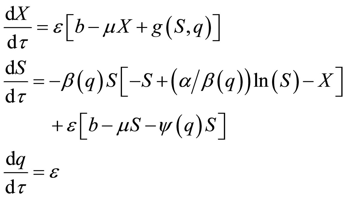
Remark 1 The attempt to have a perfect fast-slow system (in the context of singular perturbation theory) leads to a deeper examination of the function X. Note that X defines a constant on a fast system. We could heuristically define as a variable, a slow variable in the context of Singular perturbation theory. Hence we choose to transform the system to with X and S as the slow and fast variables respectively. The result is a distinct fast-slow system.

4.1. Distinct Time Scales

The system (7) mixes the slow time scales of population dynamics/vaccination with the fast time scale of the epidemic. In order to apply singular perturbation theory, we separate the time scales explicitly using a transformation of variables. The system (7) leads to the slow system,

(10)

where

Let represent the slow time, represent the fast time and The fast system reads,

(11)

Invariant Manifold

Consider the solution of model (1) on the invariant plane which corresponds to the diesease free state. This plane is also invariant for the transformed system, as the transformation is regular. In the transformed system, we denote this manifold by

The dynamics for the system where is given by the dynamics of the system where is given by It is necessary to note that neither the manifold nor the dynamics on the manifold depends on. The limiting systems, when (for the limiting fast as well as the slow system) do not have dependance, hence this manifold will be conserved. This is because if we have no infected individuals we will never have infected individuals in the system; moreover, only appears in terms that include and is not generically true for the slow manifold.

All feasible initial conditions correspond to points in

assumes values only below the maximum of The maximum is assumed at and thus .

The slow manifold generically depends on the But in this special case, hence For this reason, though is non-hyperbolic, it remains invariant nevertheless. This is generally not a feature of a non-hyperbolic manifolds.

4.2. Limiting Systems

We do the infinite separation of time, by taking to zero for the fast system. The limiting fast system reads,

(12)

We are now on the time scale of the fast process. We determine the stationary solutions of for and fixed. The two solution branches include, or

As only is allowed for we find no additional stationary points. The stationary points in the -plane are sketched in Figure 1. The dashed line indicates the unstable branch while the solid line indicates the stable branch solution. The arrows indicate the direction of the fast field.

Now consider the slow system and take to zero,

(13)

The idea is to solve for on the slow manifold given by the zero set of the function,

Let and Our focus is on systems for which the zero set of is represented by the graph of a function. That is, we assume that there exists a single-valued function, which is defined on a compact domain in such that

The zero set of thus defines a manifold in phase space,

to which the motion of the reduced slow system is confined. We note that the non-linearity of w.r.t makes it difficult to obtain the representation We are however interested in the stability along solution branches.

4.3. Stability along Slow Manifold

We read the slow manifold from the system (13) and denote it by

There are three solution branches along the slow manifold The first branch is The graph has two solution branches for herein referred to as the middle branch and which we refer to as the right hand outer branch.

In order to determine the stability along the slow manifold, we inspect the flow on the phase portrait using the nullclines of the limiting system. The branch is unstable, while branch has a stable middle branch and unstable outer branch, see Figure 1, the two branches separated at the point when the derivative of w.r.t. is equal to zero. This corresponds to the maximum point on this solution branch. On the stable part of this solution branch,

from which we define the stability threshold. Since we are on the invariant manifold the disease free solution is stable if where is defined below.

We define the instantaneous reproduction number as follows.

Definition 1 The instantaneous reproduction rate (in presence of vaccination) is defined by

We call the uninfected periodic orbit instantaneously stable, if

Note that may not be well defined for every time point, since we only know that Hence our choice of the essential supremum of this function in defining.

We note that

defined in section (3) is an average quantity over the period [0,T) while is an instantaneous stability criterion. We conjecture that there could be (for some pathological case), small epidemic outbreaks in disease even though the overall orbital stability condition still holds We reach the following conclusion.

Proposition 2 If the uninfected periodic orbit is instantaneous stable, it is also orbital stable. In general, it is not true that orbital stability implies instantaneous stability.

4.4. Defining the Optimal Control Problem Due to Instantaneous Stability

The aim is to find a vaccination schedule that is as effective as possible. During one period for vaccination we want to spend at most vaccination doses. The idea is to distribute the doses, such that the periodic solution minimizes the efficiency of this dose-distribution, measured in terms of instantaneous stability of disease free state.

Problem 2 For, find the vaccination schedule that minimizes

under the constraint that the number of vaccination doses, defined by

is bounded above by the maximum doses i.e., and the susceptible population is governed by the differential equation,

It is important to address the issue of existence for solutions for problem 4.4. We take note of the following details. One, the worst strategies maximize Furthermore, the success of any vaccination program can be defined in terms of how many susceptible individuals are still in the population, i.e., an excellent vaccination program implies no susceptible people remain in the population (all should be immune).

We therefore study vaccination strategies in terms of a set of susceptible population profiles We do not seek solutions for but do our search to a set, the closure of in [17,18].

5. Optimal Vaccination Strategies

5.1. The Set and Its Properties

In the ensuing discussion, we explore the existence of solutions within the set and by extension, in its closure For ease of notation, we shall denote the susceptible profile by We shall explore the properties of the set for purposes of existence of solutions.

Remark 2 We begin by exploring if is bounded. We also explore if the cost function in bounded. Consider the proof in the appendix Section 8. The susceptible population and the cost of vaccination are both uniformly bounded, i.e.,

and

We understand the following from where b is birth rate and T is a vaccination period. That the maximal vaccination coverage is the total new births that occur within a period of time. The actual number of vaccination doses used is thus

We further show in the appendix Section 8 that is pre-compact in and its closure is a compact subset of By this property, we can define any candidate solution in that certainly converges to a point in

Theorem 1 Let and Problem 4.4 has a solution in.

Proof. Let

As is bounded, and, the number is well defined. Consider a sequence with Suppose further that the sequence of values converges to. Since is compact w.r.t. the -topology (see appendix 8), there exists a subsequence that converge in the -norm to a point.

Suppose

That is, there is a set of non zero measure

and that there exists for which

Consider where Take. Then

The norm of the difference should not be larger than zero if converges to in the -norm. Thus, by this contradiction, we conclude that and and therefore is an optimal solution of the problem.□

We next wish to illustrate how to characterize optimal population profiles in the sense of problem 4.4.

Remark 3 The optimal vaccination strategy utilizes the least vaccination doses for maximum effect (disease control). The more the vaccination doses used, the smaller the susceptible population in the population at the end of the day. But there is a limit on how much vaccination doses we ought to use. In fact, the less vaccination doses we use, the better. The optimal vaccination solution does not correspond to the minimum susceptible population, but to the largest susceptible population for which the disease is under control, i.e. in this case, for which,

Remark 4

1) An optimal solution of problem 4.4 is a maximal element of the set

where is chosen appropriately and maximality is defined via the partial order induced by the positive cone of.

2) A maximal element of is an optimal solution of problem 4.4 at costs.

Remark 5 As the maximal element in is unique, the solution of problem 4.4 is unique.

Proposition 3 Consider any vaccination point Then the limits, and are well defined.

Proof. It follows from lemma (1) to lemma (3) in the appendix section B that the limit is well defined. In the notation in the appendix, we revert back to usual notation for susceptible solutions of our differential equation, In the sections here within the text, we have used the simpler notation to denote the solution for the susceptible population.

We now turn to the problem of how to construct optimal population profiles in an explicit manner.

Remark 6

1) We find that there are two different modes for optimal population profiles, resembling the bang-bang structure: either no control takes place and the profile behaves according to the non-controlled ODE ; or, we control enough to exactly meet the critical threshold condition.

2) This observation can be formulated in a heuristic algorithm: start at time, and note that the completely unvaccinated population has size. If, then control the population and define for small time intervals, else define. Proceed in this manner: If exceeds without control, define; if, then do not control the population, that is, define by, together with continuity requirements. If this procedure eventually leads to a periodic function, this function is a good candidate for an optimal population profile.

5.2. Candidate Optimal Vaccination Strategy

For simplicity of the function, we define two forms of periodic contact rate:

• Rectangular form, with one high and one low value within a vaccination period. This could be one calender year where contact rate is high during schooling season (assumed to be continuous with none or very short breaks) and low during holiday season (also one continuous period);

• A step function, which has high and low values in more than just two time periods.

We begin with the rectangular form of

5.2.1. Rectangular Contact Rate

It is possible to represent a two level contact rate to mimic school holidays, when contact rate is low by and school terms when the contact rate is higher by such that

Hence is periodic. Without restriction, we assume in this section always that and that the jump from to occurs at time zero and of course at time

Proposition 4 Assume that, the maximum number of vaccination doses to be used in [0,T) is fixed. The population profile for the optimal solution reads

where is to adapt to meet the requirement, and the parameter is determined by the condition

if this equation has a solution at; else, we choose.

In other words, we control the population in the first time interval; if the contact rate jumps down from to (note, that we assume), there is at least a small time window where no control is necessary. Depending on, and, it may (or may not) be the case that the population grows enough such that crosses the threshold in. Accordingly, we defined.

If we consider the vaccination rate, and not the vaccination population profile, we find that at time zero there is a delta peak, as the population necessarily jumps down to balance the jump up of the contact rate; in the next interval we control with a constant vaccination rate such that the threshold is still met. If the contact rate jumps down, no control is necessary, that is, the vaccination rate is zero. At time, we again need to control the population and have again a constant vaccination rate in the time interval. It is straight to check (or better: we check this with the considerations in this paragraph), via the proposition 5.2 that this population is optimal, indeed. We admit that proposition 5.2 requires a continuous contact rate, whereas we have here a discontinuous contact rate. However, it is (for this simple case) possible to check that the arguments still hold true.

5.2.2. Contact Rate as a Step Function

Similarly, we can handle the case of a piecewise constant function (with a finite number of jumps).

Proposition 5 Assume that, the maximum number of vaccination doses to be used in [0,T) is fixed; let be a piecewise constant function, i.e. assume that there are time points and constants such that

where

and the population profile for the optimal solution in interval reads

where is the immediate time point when is adapted to meet the requirement, and the time points are to be determined by the condition that, and on.

6. Simulation

We use simulation parameters that depict measles [19]. The population is normalized such that The death rate and birth rates are assumed equal and life expectancy is assumed to be approximately 50 years, typical of the developing countries, hence We further investigate the possible synergy between life expectancy (or residence time) and disease outbreak by considering a short residence time of only one year to match a contact or vaccination period. This rate may depict school/college stayperiods (students spend half to one year together in school or college). The constant contact rate is assumed to be per year [19]. However, we depict a periodic contact rate by a sinusoidal function that mimics a one-year period,

where year, and [20].

In Figure 2, we visualize the susceptible population profile during one year period, when we control the disease using the optimal control strategy derived from the instantaneous control problem. If we consider the number of susceptible individuals over time (upper panel), it is not clear why it follows such a time course or trajectory. But when we also consider the product, we observe that the susceptible population is controlled in such a way that this product remains constant over most part of the period, but when the product becomes smaller than a critical value, then vaccination doses are administered and then susceptible population is left to grow freely again.

In Figures 3 and 4, we now compare three different vaccination strategies: the dotted line indicates the effect of a constant vaccination rate. This is a baseline effect that we may reach without optimization. The dashed line represents the performance of the strategy optimized with respect to the instantaneous criterion, while the solid line shows the orbital optimal strategy with respect to the Floquét criterion. On the -axis of Figures 3 and 4, we have the average proportion of vaccination doses that are available for use, i.e.,

Note that this value corresponds in a one-to-one manner to the number of vaccination doses used per

period, as the costs can be represented as (see also [15]). On the -axis of Figures 3 and 4, we represent

to indicate the performance w.r.t. the Floquét stability and to denote the effect with respect to the instantaneous criterion. The functions are re-scaled in such a way that they agree with the reproduction number in case of constant contact rate and vaccination strategy and moreover, in such a way that always, is the critical threshold. Up to a certain degree, this choice of the scaling factors are arbitrary, but obvious and intuitive.

We have taken into account three different time scales in this exposition: time scale of the disease infection, given by (about one week), time scale of the contact rate and vaccination rates (about one year), and the time scale of the residence time (50 years in Figure 3 where and 1 year in Figure 4 where The central question is: how much can we gain by optimization and how much do we loose if we use the “wrong” optimization criterion?

Let us first consider a case of life expectancy of 50 years illustrated in Figure 3. We find very little difference in the effect of the optimization strategies. Somehow, the overall number of vaccination doses applied per period matters, but the timing/pattern of applying vaccination doses appears like not so important.

The scenario however improves when we consider that the residence time is in the same magnitude like the vaccination period. This situation is depicted in Figure 4. We observe a difference in this case. This effect is stronger for the instantaneous criterion than the Floquét criterion. This observation can be explained from the fact that the Floquét criterion is an average while the instanttaneous criterion considers extreme values. Thus, the extreme values that determine the supremum norm are averaged out and are less pronounced. However, for

large coverage of over 95% say, the performance of the Floquét strategy w.r.t. the instantaneous criterion is even worse than the constant strategy. In cases with a relatively short residence time, we now see that the choice of the optimization criterion obviously matters.

The fact that the critical vaccination coverage is 0.944 for the Floquét criterion and 0.963 for the instantaneous criterion is a consequence of the averaging with the Floquét term. The overall vaccination coverage necessary to eliminate the infection for a disease such as measles is always around 95%, a number that is generally hard to achieve. Especially for this reason, the organizational aspects of vaccination campaigns or vaccination days, becomes of critical importance.

7. Discussion

We investigated the influence of time scales on the stability of the uninfected solution. In the simulation, we considered the specific case of a periodic parameters including contact rate and vaccination rate. We found that the orbital stability criterion used for periodically driven systems (Floquét theory), provides an appropriate control strategy if the time scale of the disease and the contact rate are similar. If the disease is much faster (as is often the case with childhood related diseases), then singular perturbation theory defines a rather optimal control strategy; the supremum norm of the product between the susceptible population and contact rate. We used this insight to set up two different optimization problems. The first problem (the Floquét case) has been treated extensively in a different paper [15]. In this paper, we focused mainly on the instantaneous case and simulated the two strategies for comparison purposes.

The results of simulation shows that there is almost no difference in the performance of the vaccination strategies if the resident time (life expectancy) of individuals is relatively long in comparison with the period of the contact rate. This result can be also intuitively understood without the mathematical considerations: If the residence time is long, i.e., if an immunized individual lives for many time periods before he is replaced by a susceptible person again, then the importance of the time point/phase at which he is immunized does not matter. This effect is even stronger if the resident time is exponentially distributed. The results also indicate that the optimization begins (though not markedly) to matter if the residence time and the period of the contact rate do match. In this case, optimization is more important under the instantaneous criterion than under the orbital criterion, as the latter averages while the first focuses on instantaneous extreme values. The little difference in the vaccination strategies that we notice in the former case when the time scales are rather wide apart, is due to the fact that we are probably observing fast process on a slow time scale, hence we cannot see much. We must therefore separate the time scales clearly, as is the case in singular perturbation theory.

All in all, we conclusion are that in most cases, optimization will not pay if the complete population is under consideration. It only pays for small, well defined subgroups with relatively small residence times like preschool population. In this case, the importance is strengthened, from our results, by the inter-connectedness of recruitment into population, exit and contact period.

Our results support the idea of vaccination days or special vaccination periods, i.e., vaccinate when

We therefore ask whether vaccination days are beneficial, over and above constantly administering vaccination doses. Despite these results, even for large populations (larger than school populations), vaccination days may be of value. Most likely, the reason is not a certain resonance or a clever use of the interaction between the dynamics of immunization and infection, but merely an organizational effect: The way vaccination days are usually organized allows for re-vaccination such that vaccination failures are removed, and persons (mostly: children) missed in one day have the opportunity to be vaccination at another vaccination day. Moreover, the concentrated effort of vaccination (in a given location as well as in time) may enhance the interest of a large part of the population on the vaccination exercise hence the compliance becomes better. All these effects may be crucial in reaching the critical vaccination coverage that is ordinarily very difficult to reach by standard and routine means. In this sense, the result presented here should be understood as a positive result, in the sense that vaccinetion days need not to be planned only according to some dynamics of the disease but also according to organizational requirements.

8. Acknowledgements

I wish to thank the DAAD (The German Academic Exchange Program) for the support award which facilitated the completion of this research work.

REFERENCES

Appendix

The Set is Bounded and Pre-Compact in

We defined the set of optimal solutions via the set of susceptible population profiles

Interest is to show that solutions of the optimal control problem exist in this set. We therefore examine the properties of this set.

We begin by considering the following proposition.

Proposition 6 For any we find uniform bounds for and i.e.,

and

Proof. From model 1, we observe that the differential equation for the total population is,

whose solution is given by

It follows that

Since we observe that

In the new notation,

We now consider the cost functional

Consider the differential equation for the susceptible population,

Therefore,

and therefore,

To investigate compactness, we use a remark [21, p. 274] that follows from sobolev embedding theorem in [21, Theorem 1, p. 272]. We start with both the remark and the theorem (without proof as this follows from the reference).

Theorem 2 Assume is open, bounded and Lipschitz domain, s.t., Suppose then

for and

If as then

1)

for all

2)

even if

Using the above remark, we specify the following proposition.

Proposition 7 The set is a bounded subset in and is pre-compact in.

Proof. We already showed that is uniformly bounded, and thus, we only consider the bounded interval is also bounded in this interval. The norm of the derivative can be derived using the differential equation,

All the terms in the last line are uniformly bounded, i.e. is a bounded subset of. Since is compact embedded in by theorem (8), then is pre-compact in and its closure is a compact subset of

Theorem 3 If is defined for some maximal costs i.e., , the problem 3 has a solution in

Proof. is continuous functional in and the set

is non-empty and compact. Thus, the continuous functional assumes its minimum within

Convexity of

We show that is convex. According to the theorem of Krein and Milman, the extremal points structure the complete set. Consequently, we investigate this special set. The inside structure we obtain here is the centerpiece for our considerations about the structure of the optimal points in.

Proposition 8 The set is convex and so is its closure 

Proof. Let and, be population profiles in Since positive integer, we define such that, i.e.functions that stay in the positive domain and possibly bounded away from zero.

We define

Does satisfy the original differential equation for

(14)

where

(15)

Since is periodic, is also periodic, and so is By convexity of can be expressed as a convex combination of.

We also show that

Hence

Since is the closure of a convex set, it is also convex.

Hence, is a convex and compact set. The theorem of Krein-Milman [22, p. 362] tells us, that it can be characterized completely by the set of its extremal points,.

Continuity of Elements of the Set at Vaccination Points

We wish to define candidate optimal vaccination strategies that vaccinate at discrete time points. We demonstrate that the functional has well defined left hand and right hand limits at vaccination points,

Consider following Lemmata:

Lemma 1 Let be fixed and Define two functions,

Then, for

1)

2)

Proof. The set,

and denote as the measure of a set, then

Similarly,

Corollary 1 It follows that,

for arbitrarily small positive real values

Lemma 2 The exists and is equal to zero.

Proof. We know that

Thus for 

Define monotonously increasing in

Define We show that the limit exists for Suppose We know that for decreasing, is monotonously decreasing and bounded function, is monotonously increasing and bounded function, hence the following limits exist:

and

Suppose We have monotonically increasing in Since such that in the interval thus in Hence

such that as

a contradiction.

Lemma 3 exists and is equal to zero.

Proof. The proof parallels that of lemma (2), reversing time and changing the roles of the supremum and infimum.

REFERENCES

- Z. Agur, L. Cojocaru, G. Mazor, R. Anderson and Y. Danon, “Pulse Mass Measles Vaccination across Age Cohorts,” Proceedings of the National Academy of Sciences, Vol. 90, No. 24, 1993, pp. 11698-11702. http://dx.doi.org/10.1073/pnas.90.24.11698
- M. J. Ferrari, F. G. Rebecca, B. Nita, J. K. Conlan, O. N. Bjornstad, L. J. Wolfson, P. J. Guerin, A. Djibo and B. T. Grenfell, “The Dynamics of Measles in Sub-Saharan Africa,” Nature-Articles, Vol. 451, No. 7, 2008, pp. 679- 684.
- M. E. Alexander, S. M. Moghadas, P. Rohani and A. R. Summers, “Modelling the Effect of a Booster Vaccination on Disease Epidemiology,” Journal of Mathematical Biology, Vol. 52, No. 3, 2006, pp. 290-306. http://dx.doi.org/10.1007/s00285-005-0356-0
- M. Eichner and K. P. Hadeler, “Deterministic Models for the Eradication of Poliomyelitis: Vaccination with the Inactivated (IPV) and Attenuated (OPV) Polio Virus Vaccine,” Mathematical Biosciences, Vol. 127, No. 2, 1995, pp. 149-166. http://dx.doi.org/10.1016/0025-5564(94)00046-3
- P. Rohani, D. J. D. Earn, B. Finkenstaedt and B. T. Grenfell, “Population Dynamics Interference among Childhood Diseases,” Proceedings of the Royal Society of London, Vol. 265, No. 1410, 1998, pp. 2033-2041. http://dx.doi.org/10.1098/rspb.1998.0537
- P. Rohani, M. J. Kelling and B. T. Grenfell, “The Interplay between Determinism and Stochasticity in Childhood Diseases,” The American Naturalist, Vol. 159, No. 5, 2002, pp. 469-481. http://dx.doi.org/10.1086/339467
- Y. Zhou and H. Liu, “Stability of Periodic Solutions for an SIS Model with Pulse Vaccination,” Mathematical and Computer Modelling, Vol. 38, No. 3-4, 2003, pp. 299-308. http://dx.doi.org/10.1016/S0895-7177(03)90088-4
- B. Shulgin, L. Stone and Z. Agur, “Theoretical Examination of Pulse Vaccination Policy in the SIR Epidemic Model,” Mathematical and Computer Modelling, Vol. 31, No. 4-5, 2000, pp. 207-215. http://dx.doi.org/10.1016/S0895-7177(00)00040-6
- A. d’Onofrio, “Stability Properties of Pulse Vaccination Strategy in SEIR Epidemic Model,” Mathematical Biosciences, Vol. 179, No. 1, 2002, pp. 57-72. http://dx.doi.org/10.1016/S0025-5564(02)00095-0
- K. P. Hadeler and J. Mueller, “Vaccination in Age Structured Populations I: The Reproduction Number,” In: V. Isham and G. Medley, Ed., Models for Infectious Human Diseases: Their Structure and Relation to Data, Cambridge University Press, Cambridge, 1996, pp. 90-101. http://dx.doi.org/10.1017/CBO9780511662935.013
- K. P. Hadeler and J. Mueller, “Vaccination in Age Structured Populations II: Optimal Vaccination Strategies,” In: V. Isham and G. Medley, Eds., Models for Infectious Human Diseases: Their Structure and Relation to Data, Cambridge University Press, Cambridge, 1996, pp. 102- 114. http://dx.doi.org/10.1017/CBO9780511662935.014
- R. E. O’Malley, “Introduction to Singular Perturbations,” Academic Press, New York, 1974.
- R. E. O’Malley, “Singular Perturbation Methods for Ordinary Differential Equations,” Springer-Verlag, New York, 1991. http://dx.doi.org/10.1007/978-1-4612-0977-5
- N. Fenichel, “Geometric Singular Perturbation Theory for Ordinary Differential Equations,” Journal of Differential Equations, Vol. 31, No. 1, 1979, pp. 53-98. http://dx.doi.org/10.1016/0022-0396(79)90152-9
- N. Onyango and J. Müller, “Determination of Optimal Vaccination Strategies Using an Orbital Stability Threshold from Periodically Driven Systems,” Journal of Mathematical Biology, in Press. http://dx.doi.org/10.1007/s00285-013-0648-8
- H. R. Thieme, “Mathematics in Population Biology,” Princeton University Press, Princeton, 2003.
- J. Müller, “Optimal Vaccination Patterns in Age-Structured Populations,” SIAM Journal on Applied Mathematics, Vol. 59, No. 1, 1998, pp. 222-241. http://dx.doi.org/10.1137/S0036139995293270
- J. Müller, “Optimal Vaccination Patterns in Age-Structured Populations: Endemic Case,” Mathematical and Computer Modelling, Vol. 31, No. 4-5, 2000, pp. 149-160. http://dx.doi.org/10.1016/S0895-7177(00)00033-9
- B. Shulgin, L. Stone and Z. Agur, “Pulse Vaccination Strategy in the SIR Epidemic Model,” Bulletin of Mathematical Biology, Vol. 60, No. 6, 1998, pp. 1123-1148.
- N. Bacaer, M. Gabriel and M. Gomes, “On the Final Size of Epidemics with Seasonality,” Bulletin of Mathematical Biology, Vol. 71, No. 8, 2009, pp. 1954-1966. http://dx.doi.org/10.1007/s11538-009-9433-7
- L. C. Evans, “Partial Differential Equations,” American Mathematical Society, Providence and Rhodes Island, 1998.
- K. Yosida, “Functional Analysis,” Springer-Verlag, Berlin, 1980.