Communications and Network
Vol.06 No.04(2014), Article ID:51170,7 pages
10.4236/cn.2014.64022
Lyapunov Exponent Testing for AWGN Generator System
Hussein M. Hathal, Riyadh A. Abdulhussein, Sarmad K. Ibrahim
Electrical Engineering Department, College of Engineering, Al-Mustansiriya University, Baghdad, Iraq
Email: husssat@gmail.com, Riyadh_alhilali@yahoo.com, sarmad_8888@yahoo.com
Copyright © 2014 by authors and Scientific Research Publishing Inc.
This work is licensed under the Creative Commons Attribution International License (CC BY).
http://creativecommons.org/licenses/by/4.0/


Received 17 September 2014; revised 10 October 2014; accepted 20 October 2014
ABSTRACT
Additive White Gaussian Noise (AWGN) is common to every communication channel. It is statisti- cally random radio noise characterized by a wide frequency range with regards to a signal in com- munication channels. In this paper, AWGN signal is generated through design an analogue circuit method, and then the multiple recursive method is also used to generate random data signal that is used for testing by Lyapunov exponent. Furthermore an algorithm for software generating of Additive White Gaussian Noise is presented. Lyapunov exponent test for chaos is used to distin- guish between regular and chaotic dynamics of the generated data by the two methods. Simulation results are enhanced with the use of Microcontroller chip, since the hardware of the application is implemented by microcontroller-embedded system to obtain computerized noise generator. The results show that the generated AWGN signal by the analogue method and the multiple recursive method is chaotic which implies the random like-noise behavior.
Keywords:
AWGN, Chaos Technique, Lyapunov Exponent, Microcontroller-Based System

1. Introduction
White noise is a random signal (or process) with a flat power spectral density. In other words, it is the signal contains equal power within a fixed bandwidth at any center frequency. A wide band communication circuit can be measured and tested by using this noise. AWGN signal generators are hardware cost-effective, thus this ar- ticle presents a simple and inexpensive way to build white noise generators. Continuous dynamical of AWGN equations are very common in many applied sciences and engineering. Regrettably, most of these equations are nonlinear whereas most the methods of solution are linear [1] . A dynamical system is defined as a mathematical description for time evolution of a system in a state space. State space is the set of all possible states of a dy- namical system, and each state corresponds to a unique trajectory in the space. Dynamical systems can be pre- sented by attractors in phase space, and chaotic behavior sometimes occurs in these systems. In this paper, a de- scription of chaos is offered and a description of the most important indicator of chaos, the Lyapunov exponent, is offered also. The digital computer cannot generate random numbers, and it is generally not convenient to connect the computer to some external source of random events. For most applications in statistics, engineering, and the natural sciences, this is not a disadvantage if there is some source of pseudorandom numbers, samples of which seem to be randomly drawn from some known distribution. There are many methods that have been sug- gested for generating such pseudorandom numbers [2] . The multiple recursive generator (MRG), which is based on a kth-order linear recurrence relation with a large prime modulus p, has become increasingly popular in re- cent years [3] . Maximum-period Multiple Recursive Generators (MRGs) of order k have become popular pseudo- random number generators (PRNGs) in many areas of applications because of the great properties of equidistri- bution over spaces up to k dimensions, long periods, and excellent empirical performances [4] . The performance of an MRG depends on the associated order k, the prime modulus p, and the multipliers used in the recurrence equation [3] . For random numbers to be useful in general applications, their distribution must be known, and they usually must be identically and independently distributed (i.i.d.) [2] . Each sample is generated in response to the user’s request, so the samples are unique. Physical processes on the user’s computer can also be used to generate random data. There are many ways to do this. For example, Davis, Ihaka, and Fenstermacher (1994) describe a method of using randomness in the air turbulence of disk drives [2] . A basic and generally accepted model for thermal noise in communication channels is the set of assumptions that:
· The noise is additive, i.e., the received signal equals the transmit signal plus some noise, where the noise is statistically independent of the signal.
· The noise is white, i.e., the power spectral density is flat, so the autocorrelation of the noise in time domain is zero for any non-zero time offset.
· The noise samples have a Gaussian distribution. The operation of the analogue system is based on the noise generated by the Zener breakdown phenomenon in an inversely polarized diode as shown in Figure 1 [1] .
2. Generation of Random Numbers
Since many statistical methods rely on random samples, applied statisticians often need a source of “random numbers”. The use of random numbers in statistics has expanded beyond random sampling or random assign- ment of treatments to experimental units [2] . The digital computer cannot generate random numbers, and it is ge- nerally not convenient to connect the computer to some external source of random events. There are many me- thods that have been suggested for generating pseudorandom numbers.
2.1. Multiple Recursion Method
It is the most useful type of generator of pseudorandom processes updates a current sequence of numbers in a manner that appears to be random. Such a deterministic generator, f, yields numbers recursively, in a fixed se- quence. The previous k numbers (often just the single previous number) determine(s) the next number [5] :

The number of previous numbers used, k, is called the “order” of the generator. The set of values at the start of the recursion is called the seed. Each time the recursion is begun with the same seed, the same sequence is generated. The length of the sequence prior to beginning to repeat is called the period or cycle length. The stan- dard methods of generating pseudorandom numbers use modular reduction in congruential relationships. There are currently two basic techniques in common use for generating uniform random numbers: congruential me- thods and feedback shift register methods. The basic relation of modular arithmetic is equivalence modulo m, where m is some integer. This is also called congruence modulo m. Two numbers are said to be equivalent, or

Figure 1. Additive white Gaussian noise generator system.
congruent, modulo m if their difference is an integer evenly divisible by m. For a and b, this relation is written as [4] [5] :

A simple extension of the multiplicative congruential generator is to use multiples of the previous k values to generate the next one:
 (1)
(1)
When k > 1, this is sometimes called a “multiple recursive” multiplicative congruential generator. The number of previous numbers used, k, is called the “order” of the generator. (If k = 1, it is just a multiplicative congruen- tial generator). The period of a multiple recursive generator can be much longer than that of a simple multiplica- tive generator.
2.2. Additive White Gaussian Noise Generator Method
In every communications channel noise is always present. Furthermore, other disturbances which cause the transmitted signal to change, such as fading, may also be present. In most cases, AWGN is used to evaluate the performance of a communication system in a noisy channel [6] . Additive white Gaussian noise (AWGN) is a channel model in which the only impairment to communication is a linear addition of wideband or white noise with a constant spectral density (expressed as watts per hertz of bandwidth) and a Gaussian distribution of am- plitude. The model doesn’t account for fading, frequency selectivity, interference, nonlinearity or dispersion. However, it produces simple and tractable mathematical models which are useful for gaining insight into the underlying behavior of a system before these other phenomena are considered. Wideband Gaussian noise comes from many natural sources, such as the thermal vibrations of atoms in conductors (referred to as thermal noise or Johnson-Nyquist noise), shot noise, black body radiation from the earth and other warm objects, and from celes- tial sources such as the Sun [1] . The AWGN channel is a good model for many satellite and deep space commu- nication links. It is not a good model for most terrestrial links because of multipath, terrain blocking, interference, etc. However, for terrestrial path modeling, AWGN is commonly used to simulate background noise of the channel under study, in addition to multipath, terrain blocking, interference, ground clutter and self-interfer- ence that modern radio systems encounter in terrestrial operation.
3. Description of Chaos
The greatest power of science lies in its ability to relate causes to effects. The evolution of a dynamical system may occur either in continuous time or in discrete time. The former is called flow, and the latter is called map. For nonlinear systems, continuous flow and discrete map are also two mathematical concepts used to model chaotic behavior [7] . Chaos can be observed in a time series or in a phase space plot, but this is not very accurate. At present, there are a number of methods employed to detect chaos in dynamical systems, such as power spec- trum analysis, the 0 - 1 test, calculating the Lyapunov exponents, and so on.
Lyapunov Exponent
The Lyapunov exponents of a system under consideration characterise the nature of that particular system. They are perhaps the most powerful diagnostic in determining whether the system is chaotic or not. Furthermore, Lyapunov exponents are not only used to determine whether the system is chaotic or not, but also to determine how chaotic it is. The Lyapunov exponents characterise the system in the following manner. Suppose that do is a measure of the distance among two initial conditions of the two structurally identical chaotic systems. Then, af- ter some small amount of time the new distance is [8] :
 (2)
(2)
where  denotes the Lyapunov exponent.
For chaotic maps, Equation (2), is rewritten in the form of Equation (3):
 (3)
(3)
where  denotes the Lyapunov exponent and n a single iteration of a map. The choice of base 2 in Equations (2) and (3) is arbitrary [8] . The Lyapunov exponents of Equations (2) and (3) are known as local Lyapunov ex- ponents as they measure the divergence at one point on a trajectory (orbit). In order to obtain a global Lyapunov exponent the exponential growth at many points along a trajectory (orbit) must be measured and averaged. The largest Lyapunov exponents of a dynamical system have been developed to be the most important number of invariants, for characterizing chaos. Mathematically, the Lyapunov exponent of a dynamical system is a measure that used to characterize the rate of separation of infinitesimally close trajectories [9] . The Lyapunov exponent is used also to determine the level of chaos within it. In order to determine a global Lyapunov exponent, the expo- nential growth at many points along an orbit must be calculated and then averaged. The largest Lyapunov expo- nent is described as [2] [7] [9] :
 (4)
(4)
where  means the growth rate of the distance between neighboring trajectories. And the largest lya- punov exponent
  for chaotic maps is described by Equation (5):
 (5)
(5)
where .
.
A dynamical system is said to be chaotic if the Lyapunov exponent  is positive (larger than zero). When the Lyapunov exponent
  is negative, this implies that the dynamical system is a fixed point or a periodic cycle. For a chaotic system, there are many Lyapunov exponent equal to its dimension. The logistic map (one dimensional map) given by:
 (6)
(6)
has a one positive Lyapunov exponent. The Hénon map (two dimensional maps) of has two Lyapunov expo- nents, one positive and the other negative. The Lorenz chaotic flow of (three dimensional maps) has three Lya- punov exponents, one positive, one negative and one equal to zero [2] [7] .
4. Testing of Random Noise Generator Results Based on Chaos Technique
If all of the relevant information in the system is well known, the calculation of the theoretical Lyapunov expo- nents can be based on the equations of that system. This method includes repeatedly using equation linearization. In reality, the equations in a given system are not easy to obtain. However, time series data sets can easily be acquired. When only time series data are recorded, the calculation method introduced above is impossible to use. Alan Wolf [8] offers an algorithm to use in order to compute the LLE from time series data. Moreover, the di- mension and origin of the dynamical system [3] and the form of the underlying equations are irrelevant. The in- put is the time series data and the output is 0 or 1, depending on whether the dynamics is non-chaotic or chaotic. The test is universally applicable to any deterministic dynamical system.
Description of the Lyapunov Exponent Test Algorithm for Chaos
This procedure can briefly be summarized as follows:
1) Choose and put the initial values of the multiple recursive method.
2) Calculate the next step of the multiple recursive method.
3) Calculate the derivative of the multiple recursive equation.
4) Calculate Lyapunov exponent value.
5) Calculate the Largest value of Lyapunov exponent, .
.
6) Test the  value.
7) If > 0, then the system behavior is chaotic, and if <0, then the system behavior is periodic (i.e., non-chao- tic).
The flow chart for calculating Lyapunov exponent values is shown in Figure 2.
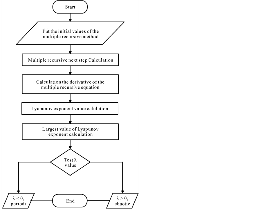
Figure 2. Flow chart of Lyapunov exponent test algorithm for chaos.
5. AWGN Generator Simulation Results
In this section, the simulation results are given to verify the theoretical results by implementing the AWGN ge- nerator system of Figure 3. The data that used for testing is generated by applying the multiple recursive method through the PIC microcontroller chip, and then it tested by using Lyapunov exponent chaos test.
The noise amplitude versus the number of samples is obtained by applying the multiple recursive method as shown in Figure 4, while Figure 5 represents the amplitude of the power spectral density opposes the number of samples.
In order to test the AWGN signal that is generated by the PIC microcontroller, so Lyapunov exponent chaos test is applied. When the time series data, i.e., AWGN signal, is entered as vector of values, then an embedding lag of state space reconstruction is initialized such that an embedding dimension must be calculated. If embed- ding dimension be selected correctly, then there would have smooth part (or fairly horizontal) on the Lyapunov exponent curve. So if there is no smooth section on the curve, it is better to try with other embedding dimensions. When there is not any information about proper value of embedding dimension, then should let it zero (0). In this case code automatically selects proper m by False Nearest Neighbors (or FNN) method, if this method fails due to high noise in data, the code will use another method named symplectic geometry. This method is a gra- phical in nature however it use test for selection of vector based on variance change of eigenvalues. The sym- plectic geometry method for determination embedded dimension is shown in Figure 6.
Figure 7 illustrates the nonlinear regression Layapunov exponents, for multiple recursive method the Lyapu- nov exponent  is positive (i.e., larger than zero) therefore, the generated data is chaotic. Also, for AWGN generator, the Layapunov exponents took positive values therefore; the generated data is chaotic too.
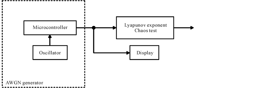
Figure 3. Block diagram of AWGN generator testing system.
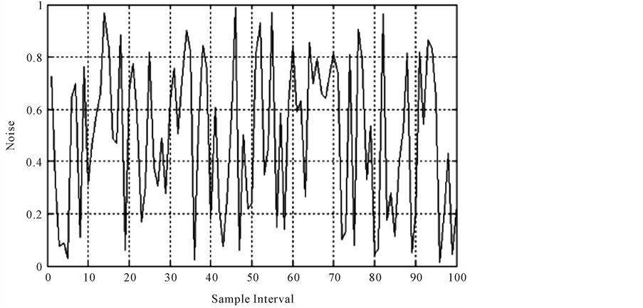
Figure 4. Noise amplitude versus number of samples.
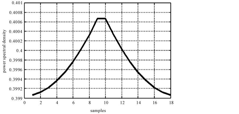
Figure 5. Power spectral density amplitude versus number of samples.
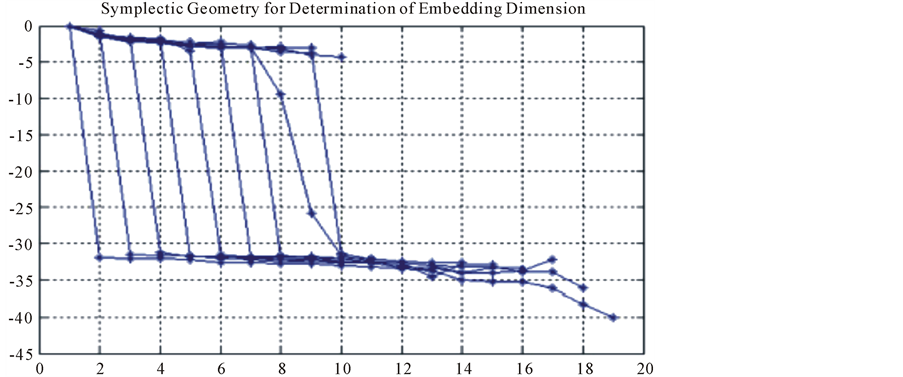
Figure 6. Symplectic geometry method for determination embedded dimension.
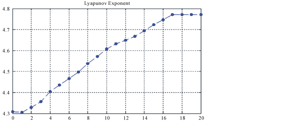
Figure 7. Large Lyapunov exponent for AWGN signal generated by multiple recursive method.
6. Conclusions
Chaos is a developing research topic. In this paper, Lyapunov exponent test for Multiple Recursive Method and additive white Gaussian noise generator is implemented. The application of Lyapunov exponent in real world dynamical systems is rarely developed. So, the method of testing by using Lyapunov exponent is proposed in this paper work. In order to obtain Lyapunov exponent from the experimental AWGN time series data, a method mainly based on phase space reconstruction is demonstrated. The phase space reconstruction requires a time de- lay and an embedding dimension. The digital software implementation of AWGN generators achieved; reliabil- ity and accuracy, where digital circuits have more reliability than analogue circuits, and wide number generation range, so in digital circuits, the range of random numbers is more wide than the range of random numbers ob- tained by analogue circuits, since there are various algebraic methods can be implemented by software.
Lyapunov exponent test for chaos is used for the analysis of nonlinear discrete and continues deterministic dynamical systems, the test distinguish between regular and chaotic dynamics. This distinction is extremely clear by means of the diagnostic variable , which has values either positive or negative. In particular the equ- ations of the underlying dynamical system do not need to be known, and there is no practical restriction on the dimension of the underlying vector field. Simulation results show that the AWGN signal that is generated by the Multiple Recursive Method behaves randomly and can be used in simulating real world applications.
References
- Xiao, P. (2009) Effect of Additive White Gaussian Noise (AWGN) on the Transmitted Data. 1-15.
- Gentle, J.E. (2003) Random Number Generation and Monte Carlo Methods. 2nd Edition, Springer, Berlin.
- Deng, L.-Y., Shiau, J.-J.H. and Shing Lu, H.H. (2011) Large-Order Multiple Recursive Generators with Modulus 231- 1. INFORMS Journal on Computing, 1-12.
- Deng, L.-Y., Shiau, J.-J.H. and Shing Lu, H.H. (2012) Efficient Computer Search of Large-Order Multiple Recursive Pseudo-Random Number Generators. Journal of Computational and Applied Mathematics, 236, 3228-3237. http://dx.doi.org/10.1016/j.cam.2012.02.023
- Giacobazzi, R. and Ranzato, F. (1998) Some Properties of Complete Multiple Recursive Lattices. Algebra Universe, 40, 189-200.
- Jovic, B. (2011) Synchronization Techniques for Chaotic Communication Systems. Springer, Berlin. http://dx.doi.org/10.1007/978-3-642-21849-1
- Aziz, M.M. and Faraj, M.N. (2012) Numerical and Chaotic Analysis of CHUA’S CIRCUT. Journal of Emerging Trends in Computing and Information Sciences, 3.
- Alligood, K.T., Sauer, T.D. and Yorke, J.A. (1996) Chaos: An Introduction to Dynamical Systems. Springer, Berlin.
- Sun, Y. (2011) Fault Detection in Dynamic Systems Using the Largest Lyapunov Exponent. Thesis, Texas.