Open Journal of Air Pollution
Vol.07 No.03(2018), Article ID:86761,29 pages
10.4236/ojap.2018.73011
PM2.5 Estimation with the WRF/Chem Model, Produced by Vehicular Flow in the Lima Metropolitan Area
Warren Reátegui-Romero1,2, Odón R. Sánchez-Ccoyllo1,3, María de Fatima Andrade4, Aldo Moya-Alvarez5,6
1School of Sciences, Universidad Nacional Agraria La Molina (UNALM), Lima, Peru
2School of Chemical Engineering and Textile (FIQT), Universidad Nacional de Ingeniería (UNI), Rímac, Lima, Peru
3School of Environmental Engineering, Universidad Nacional Tecnológica deLimaSur (UNTELS), Villa El Salvador, Lima, Peru
4Department of Atmospheric Sciences at the Institute of Astronomy, Geophysics and Atmospheric Sciences (IAG), University of São Paulo, São Paulo, Brazil
5Centro Meteorológico Provincial Santa Clara, Cuba
6Instituto Geofísico del Peru (IGP), Calle Badajoz N˚ 169 Urb. Mayorazgo IV Etapa Ate, Lima, Peru

Copyright © 2018 by authors and Scientific Research Publishing Inc.
This work is licensed under the Creative Commons Attribution International License (CC BY 4.0).
http://creativecommons.org/licenses/by/4.0/


Received: June 13, 2018; Accepted: August 18, 2018; Published: August 21, 2018
ABSTRACT
Lima is the capital of the Republic of Peru. It is the most important city in the country and as other Latin America metropolises have multiple problems, including air pollution due to particulate material above air quality standards, emitted by 1.6 million vehicles. The “on-line” coupled model of meteorology and chemistry of transport and meteorological/chemistry, WRF/Chem (Weather and Research Forecasting with Chemistry) has been used in the Lima Metropolitan Area, and validated against data observed at ground level with ten air quality stations of the National Service of Meteorology and Hydrology for the year 2016. The goal of this study was to estimate the concentration of PM2.5 particulate matter in the months of February and July of 2016. In both months, the model satisfactorily predicts temperature and relative humidity. The average observed PM2.5 concentrations in the month of July are higher than in February, probably because the relative humidity in July is greater than the relative humidity in February. In the months of February and July the standard observed deviations of the model have a factor of 2.4 and 3.7 respectively, indicating a greater dispersion in the data of the model. In the month of July, the model captures the characteristics of transport, shows characteristic peaks during peak hours, therefore, the model estimates transport behavior better in July than in February. The quality of the air is strongly influenced by the vehicular transport. The PM2.5 particulate material in February had an average bias that varied from [−13.2 to 4.4 μg/m3] and in July [−9.63 to 11.65 μg/m3] and a normalized average bias in February that varied from [−0.68 to 0.43] and in July of [−0.46 to 0.48].
Keywords:
Air Quality, Aerosol, WRF/Chem Model, PM2.5, Lima-Peru

1. Introduction
Lima is the capital of the Republic of Peru. It is located on the country’s central coast, on the shores of the Pacific Ocean at 77˚W and 12˚S. The Lima Metropolitan Area (AML) is the most extensive and populated metropolitan area of Peru, with 2819.3 km2 [1] , a population of 10.4 million inhabitants [2] and 1674,145 million vehicles [3] ; (http://www.inei.gob.pe/). Cities with over 10 million inhabitants are considered megacities [4] [5] [6] [7] . These megacities are the engines of growing economies, but are also very large sources of air pollutants and climate-forcing agents [8] . Uncontrolled urban sprawl has led to rising environmental problems due to high traffic volume, irregular industry, etc. [5] . The growing problems of congestion, accidents, and lack of security are also worrisome. Yet transportation is also a critical enabler of economic activity and beneficial social interactions [9] . Transportation is a major source of air pollution in many cities [9] [10] , especially in developing countries [9] . Air quality at urban background sites is strongly influenced by road traffic emissions, which is the most important emission source concerning its contribution to ambient PM levels [11] [12] . Emitted primary and subsequently formed secondary gas- or particulate-phase pollutants [13] , cause substantial health problems especially in megacities with rapidly growing industry and low pollution control [7] [14] . Particles in the atmosphere arise from natural sources, such as windborne dust, sea spray, and volcanoes, and from anthropogenic activities, such as fuel combustion. Whereas an aerosol is technically defined as a suspension of fine solid or liquid particles in a gas [15] , atmospheric particulate matter (PM) is one of the primary concerns in megacities, due to their association with health effects and environment problems [16] [17] . Particulate air pollution is a mixture of solid particles and liquid droplets that vary in size, composition, and origin. Only very small particles can be inhaled into the lungs, inhalable particles include particles with an aerodynamic diameter of less than 10 µm, and fine particles; air pollution includes particles with an aerodynamic diameter equal to or below 2.5 µm [16] [18] . Deterioration in urban environmental conditions can have serious effects on human health and welfare, particularly for the poor [9] . Epidemiological studies suggest that exposure to (PM2.5 and PM10) atmospheric particulate matter can cause adverse effects, including coughing, respiratory stress in asthmatics, and reduced lung function [17] , bronchitis, and conjunctivitis [19] . These studies have also shown that air pollution exposure is related with general morbidity and mortality due to respiratory and cardiovascular diseases [18] [19] . The ambient air in Peru is contaminated at a high level compared to other Latin American countries, according to a report by the World Health Organization (WHO) [20] . Lima is the only municipality reporting to the World Health Organization and has high levels of particulate matter contributing to poor air quality. Short term symptoms resulting from exposure to air pollution include itchy eyes, nose and throat, wheezing, coughing, shortness of breath, chest pain, headaches, nausea, and upper respiratory infections (bronchitis and pneumonia). It also exacerbates asthma and emphysema. Long term effects include lung cancer, cardiovascular disease, chronic respiratory illness, and developing allergies. Air pollution is also associated with heart attacks and strokes [21] . A study that relates the impact of vehicle flow with adolescent asthma in the city of Lima can be consulted in [22] , while in [23] , some Peruvian cities with PM air pollution problems are indicated. Problems of indoor air pollution in the periurban community of Lima by vehicular transport can be consulted in [24] . Deficiencies in public transport, as well as air pollution and proposals for improvements for transportation in Lima can be consulted in [25] . The poor air quality in the AML and its relationship with human deaths and other health problems that affect the population due to PM and other air pollutants, can be reviewed in [26] [27] , and [28] . The goal of this study was to estimate the PM2.5 particulate matter concentration in the Metropolitan Area of Lima (AML) using the Eulerian WRF-Chem Model, in the months of February (summer) and July (winter) and was validated with measurements at ground level in the ten air quality stations of the National Service of Meteorology and Hydrology (SENAMHI) Lima, Peru. In order to improve the results of the model’s output, the MOS statistical technique was applied. Model Output Statistics (MOS) is a type of statistical post-processing, a class of techniques used to improve numerical weather models’ ability to forecast by relating model outputs to observational or additional model data (https://www.weather.gov/mdl/mos_home) [29] . The MOS was defined by [30] as a multiple linear regression technique in which predicands (observed data) are statistically related to one or more predictors (forecasts from a numerical weather prediction (NWP) model).
2. Methodology
2.1. Study Area
The study area corresponds to the AML, that is located at coordinates (Longitude: 77˚1'41.66W, Latitude: S12˚2'35.45S). The air quality data was provided by the ten monitoring stations of the National Service of Meteorology and Hydrology of Peru (SENAMHI). In Lima, climate is very peculiar: it is a subtropical desert climate, with a warm season from December to April, and a cool, humid, and cloudy season from June to October, with May and November as transition months. During summer, from December to April, sunshine is frequent, at least during the warmest hours of the day, while in the early hours of the day, fog may still form. Even in this season, at times banks of low clouds can form, though that is more rarely. The temperature is pleasantly warm. During winter, from June to September, the sky is almost always cloudy, and there is a kind of mist, garúa [drizzle], which can leave a bit of moisture on the ground. Temperatures are mild, but the lack of sunshine and high air humidity increase the feeling of coldness, also because houses are not heated. Thermal inversion favors the accumulation of pollutants on the ground, despite the proximity to sea (https://www.climatestotravel.com/climate/peru/lima). The meteorological data is reported in the Jorge Chavez International Airport (http://www.enperu.org/clima-capital-de-peru-lima-temperaturas-ciudad-de-lima-altitud-latitud-capital-peru.html). The average annual temperature is 19˚C with an annual summer maximum close to 29˚C. Summers, from December to April, have temperatures that range between 21˚C and 29˚C. Winters go from June to mid-September with temperatures ranging between 12˚C and 19˚C [31] . Figure 1 shows the location of the air quality stations on AML and Table 1 indicates the coordinates of these stations of the National Service of Meteorology and Hydrology of Peru (SENAMHI).
2.2. Observed Data
The equipment used by the National Meteorology and Hydrology Service of Peru (SENAMHI), for the data collection, was the TEOM 1405 monitor and Model 5014i Beta Continuous Ambient Particulate Monitor. The TEOM 1405 monitor uses a Tapered Element Oscillating Microbalance (TEOM) to provide measurements with excellent short-term precision and account for volatile and nonvolatile PM fractions. “The TEOM 1405 Monitor is a real-time device used for measuring the particulate matter mass concentration of particulate matter”. “The

Table 1. Location of air quality monitoring stations of the National Service of Meteorology and Hydrology of Peru: SENAMHI-Lima.
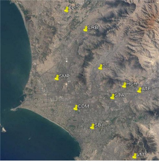
Figure 1. Geographical location of SENAMHI-Lima air quality stations.
TEOM 1405 Monitor is a true gravimetric instrument that draws (then heats) ambient air through a filter at constant flow rate, continuously weighing the filter and calculating near real-time mass concentrations of particulate matter”. “The tapered element at the heart of the mass detection system is a hollow tube, clamped on one end and frees to oscillate at the other. An exchangeable TEOM filter cartridge is placed over the tip of the free end. The sample stream is drawn through this filter, and then down the tapered element. This flow is maintained at a constant volume by a mass flow controller that is corrected for local temperature and barometric pressure” [32] . In this study the TEOM 1405 monitor was used to measure the mass concentration of PM10. “The Model 5014i uses the radiometric principle of beta attenuation through a known area on a fibrous filter tape to continuously detect the mass of deposited ambient particles. Additionally, the Model 5014i measures alpha particle emissions directly from the ambient aerosol being sampled and excludes negative mass artifacts from the daughter nuclides of radon gas decay to achieve a refined mass measurement. Simultaneous refined mass measurements of sampled particulate on the filter tape and sample volume measurement provide a continuous concentration measurement of ambient particulate concentration” [33] . In this work the Model 5014i Continuous Ambient Particulate Monitor continuously measures the mass concentration of PM2.5 by the use of beta attenuation.
At each station, the available PM2.5 information was greater than 75%. The percentage of observed and [32] used PM2.5 data on a 29-day basis at each station in the month of February was (CDM: 0%, ATE: 90.80%, SBJ: 100%, STA: 100%, CRB: 86.10%, HCH: 81.90%, PPD: 78%, SMP: 86.20%, VMT: 0% and SJL: 100%), and in the month of July, it was (CDM: 100%, ATE: 90.80%, SBJ: 80.32%, STA: 0%, CRB: 89.84%, HCH: 0%, PPD: 100%, SMP: 93.55%, VMT: 93.55% and SJL: 100%).
2.3. Model of Anthropogenic Emissions in the AML
Because on-road vehicles are the most important sources of air pollution in AML, according to DIGESA, more than 78% of pollutant emissions are generated by vehicular emissions; the anthropogenic emissions of trace gases and particles in 5 km modeling domains were considered to include emissions only coming from on-road vehicles through the use of a vehicular emission model [34] . Then, vehicular emission in the AML for the WRF-Chem Model was estimated using a Vehicular Emission Model-VEM developed by the IAG-USP’s Laboratory of Atmospheric Processes-LAPAt [34] . “This VEM model does not include point sources nor biogenic sources, and considers the number of vehicles, vehicular emissions factors, and average driving kilometers for vehicle per day as basic parameters for the calculations of exhaust and evaporative emissions considering different vehicles types and different fuel types” [34] . “For the spatial distribution of air pollution emissions, it is assumed that the vehicles within the modeling domain were distributed proportional to the road length in each grid cell” [12] [13] [35] . “Road length was calculated as the sum of five types of road (motorway, trunk, primary, secondary and tertiary) within each grid cell” [36] . “The road map is available on the Open Street Map project and extracted from the Geofabrik’s free download server (http://download.geofabrik.de/)” [36] .
2.4. Description and Configuration of the WRF/Chem Model
WRF-Chem is the Weather Research and Forecasting (WRF) model coupled with chemistry [37] . The model simulates the emission, transport, mixing, and chemical transformation of trace gases and aerosols simultaneously with meteorology. The model is used for investigation of regional-scale air quality, field program analysis, and cloud-scale interactions between clouds and chemistry (https://www2.acom.ucar.edu/wrf-chem); WRF is non-hydrostatic [38] [39] , with several dynamic cores as well as many different choices for physical parameterizations to represent processes that cannot be resolved by the model [37] . The WRF physics and chemical options fall into several categories, each containing several choices. The physics categories are: microphysics, cumulus parameterization, planetary boundary layer (PBL), land-surface model, atmospheric radiation, and diffusion [40] . The chemical categories are: several choices for gas-phase chemical mechanisms, photolysis schemes, aerosol schemes etc. [41] . To know which organizations participated in the design of the model, you can consult [42] [43] . For the implementation of WRF/Chem, the initial and frontier conditions of the Global Prediction System (GFS) were used (see Table 2). The predicted data were used for each day at 00:00, 06:00, 12:00 and 18:00
Table 2. Main characteristics of the domain and initial and frontier data.
hours of Coordinated Universal Time (UTC) (http://rda.ucar.edu/datasets/ds083.3/). This product is from the Global Data Assimilation System (GDAS), which continuously collects observed information from the Global Telecommunications System (GTS), and other sources for analysis. The analyses are available on the surface, at 27 mandatory levels of pressure, from 1000 millibars at sea level to 10 millibars in the boundary layer. Parameters include surface pressure, sea level pressure, geopotential height, temperature, sea surface temperature, soil values, ice sheet, relative humidity, zonal winds (u), and southern (v), vertical movement, vorticity, and ozone. (http://rda.ucar.edu/datasets/ds083.3/). In Table 2 the characteristic “DC Frequency (Frequency of Contour Conditions)” refers to the frequency with which the boundary conditions are captured from the output of the base model, in this case, the GFS. Version 3.8.1 of the WRF/Chem air quality model was used for this study over AML [35] . The physical and chemical parameterization schemes used in this study are shown in Table 3. Details can be found in [35] [40] .
With respect to the configuration model, the following studies can be consulted: on short-wave radiation and long-wave radiation [44] and [45] respectively, on planetary boundary layer (YSU) [46] , on land-surface model [47] , on cumulus cloud [48] , on cloud microphysics [49] , on photolysis scheme (Fast-J) [50] , on gas-phase mechanism (RADM2) [51] , and on aerosol option (MADE/SORGAM) [52] . This configuration does not consider point emissions or biogenic emissions.
2.5. Statistical Models and Improvement of the WRF-Chem Prognosis with MOS
The mean bias (MB), normalized mean bias (NMB), and RMSE (Root Mean Squared Error) were used to evaluate the model performance in simulating aerosols [53] [54] [55] .
(1)
(2)
Table 3. Configuration of the WRF-Chem for the simulations in Lima.
(3)
where Xoi and Ypi are the average hourly observed and predicted data respectively. In this study, a linear regression with a linear function was used to calculate the regression coefficients, which are used to improve the prognosis. However, it is also possible to use linear regression with non-linear functions of the variables. The hourly values of the model Yp, have been improved by applying the MOS technique. The procedure is:
(4)
(5)
where a and b are the coefficients of the linear regression. Ynpi represents the improved value of the forecast. This scheme allowed us to generate new information for each station, whose profiles are shown in Figures 7-16.
3. Results and Discussion
3.1. Characterization of Meteorological Data of the Global Forecasting System (GFS) for the Months of February and July 2016 for Boundary and Initial Conditions of the Eulerian Model WRF-Chem in the AML
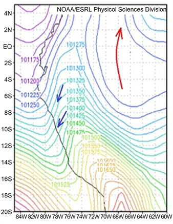
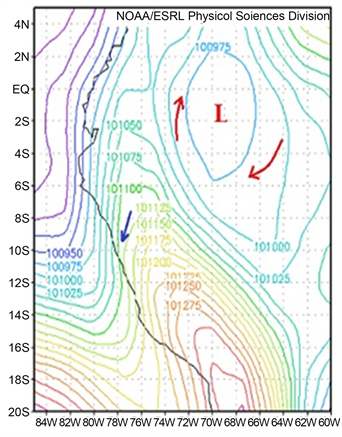
Figure 2 shows the average fields of pressure at the mean sea level for the months of February (a) and July (b). In a general sense, it can be seen that there are no large differences in the circulation of air at low levels, and in both cases the predominant general flow in Lima is from the northeast. However, under certain conditions, local circulation may temporarily occur during the day, the general circulation varying to a certain extent.
 (a) (b)
Figure 2. Average pressure fields at the mean sea level for the months of February (a) and July (b).
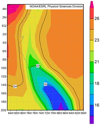
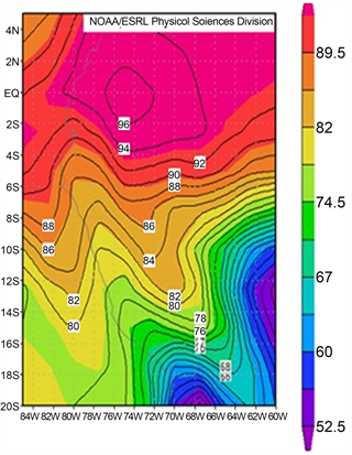
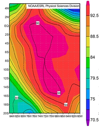
Figure 3 shows the temperature field for the region, clearly marking a high thermal gradient between the coast and the mountain range. In this case, the temperatures over the AML in February (summer) vary between 20˚C and 21˚C, higher than in July (winter), below 19 ˚C. Figure 4 shows the average moisture values in the AML. In February and July the values oscillate around 93% and 82% respectively.
3.2. Temperature and Relative Humidity
Table 4 shows average temperatures and relative humidity predicted in the months of February (summer season) and July (winter season) for the ten monitoring stations. In February, global average values in the AML were 20.42˚C ± 1.25˚C and 76.86% ± 8.10% respectively. The range of variation of these parameters were from [15.86 a 24.33˚C] and [47.06% to 100%] respectively. In the month of July (winter season) these average values were of 17.61˚C ± 1.11˚C and 80.11% ± 5.60% respectively, with ranges of [13.03˚C to 23.49˚C] and [50.38% to 98.08%].
Figure 5 and Figure 6 show the average predicted and observed monthly temperature profiles for February and July at the CMD station. The model in February has a better performance than in July, which is corroborated by the statistical parameters with values closer to zero that are shown in Table 5, in July the model underestimates the observed data. In February the observed average daily values of temperature and relative humidity were 24.75˚C and 79.02% respectively, with ranges of [23.55˚C to 26.27˚C] and [72.46% to 83.96%], and the values predicted averages were 21.29˚C, and 77.38% respectively with ranges of [20.39˚C to 22.14˚C] and [68.66% to 82.94%]. In the month of July, the average

 (a) (b)
Figure 3. Average surface temperature fields for the months of February (a) and July (b).
 (a) (b)
Figure 4. Average relative humidity fields on the surface for the months of February (a) and July (b).
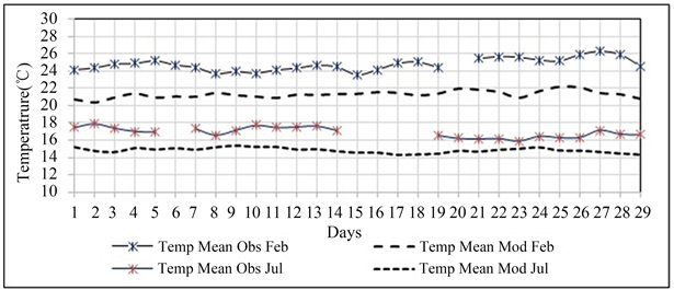
Figure 5. Temperature profiles observed and predicted from average values at the CDM station in February and July.
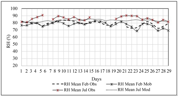
Figure 6. Average relative humidity profiles of observed and predicted values at the CDM station in February and July.
Table 4. Summary of the average hourly estimate of the temperatures and relative humidity of February and July. The standard deviation SD is with respect to the average value.
Table 5. Average monthly statistics MB, NMB and RSME of temperature ˚C and RH% in the CDM station.
values were of 16.87˚C and 84.08% with ranges of [15.90˚C to 17.89˚C] and [80.67% to 90.91%] respectively, and the predicted average values were of 14.85˚C and 83.17% with ranges from [15.82˚C to 13.77˚C] and [64.04% to 94.57%] respectively.
At the Alexander Von Humboldt Meteorological Station (location: 12˚4'55"S 76˚56'20"W) of the National Agrarian University La Molina in the month of February, the average observed values of temperature and relative humidity were of 26.00˚C and 76.00%, and their ranges were from [21.80˚C to 29.90˚C] and [89.00 to 99.00%] respectively, and in the month of July the average values were 17.00˚C and 88.20%, with ranges of [14.7˚C to 19.7˚C] and [78.8% to 96.9%] respectively.
At the Jorge Chavez International Airport meteorological station average values of temperature and relative humidity in the month of February were 25˚C and 79%, with ranges of [19˚C to 30˚C] and [49% to 100%] respectively, and in July these average were 17˚C and 83% and their ranges were [15˚C to 20˚C] and [68% to 96%] [56] . In the AML, the temperature and relative humidity in summer fluctuate in a range of 21˚C to 29˚C and 70% to 90% respectively, and in winter these parameters vary from 15˚C to 19˚C and 80% to 90% respectively [31] .
3.3. Comparison Factors of Modeling and Observed PM2.5
Table 6 shows the PM2.5 Mod/PM2.5 Obs and PM2.5 MOS/PM2.5 Obs factor at each station and month. There are no observed PM2.5 data at the CDM and VMT stations in the month of February, in the same way at the ATE, STA and VMT stations in July. If the factor is greater or less than unity, the model in general overestimates and underestimates the observed data. As expected, February and July, this factor improved with the MOS as values got closer to the unit, except in the case of the CRB station for July, this shows that if the model does not perform well the MOS will improve the predicted data but not too much.
Tabla 6. Factor F1 = PM2.5 Mod/PM2.5 Obs y F2 = PM2.5 MOS/PM2.5 Obs.
3.4. Statistical Parameters MB, NMB and RMSE in February and July at the 10 Stations
Table 7 shows the MB, NMB and RMSE statistics. In general, the July values are smaller than the ones in February at the stations where it is possible to compare the statistics, with exception of RMSE in July. These values are higher than February. It can be seen that the MOS improves the forecast, since these values are close to zero.
Table 8 shows the values of the coefficients a and b calculated with equation 4 for each station in February and July. The profiles of improved average values calculated with Equation (5) are shown in Figure 7.
3.5. PM2.5 Spatial Distribution Characteristics
For the month of July, Figure 7 shows the hourly profiles of average PM2.5 values observed, modeled, and improved with MOS at the CDM station. The average concentration of the observed values decreases between 0:00 and 5:00 hours. The model captures this detail underestimating it. After 06:00 the model overestimated the observed data showing two marked peaks of vehicular traffic at peak hours.
The MOS, represented as a dotted line, as expected has a better response, as its values are around the observed average values as shown by its statisticians. The peak hours in the AML have been marked from 07:00 to 09:00 hours [57] , and from 18:00 to 20:00 hours [58] . The average values observed in July, predicted and improved with the PM2.5 MOS were 14.83 ± 2.32, 19.25 ± 12.53, and 14.70 ± 0.59 μg/m3 respectively. Other studies in winter show that the observed and predicted average values were 36.0 and 18.1 μg/m3 [59] . In this case the model underestimated the observed data. The mean bias (MB) varied in a range of [−10.71 to 28.92 μg /m3], which indicates that the model underestimated and overestimated the observed data and its average value was 4.42 ± 12.18 μg/m3. In others studies in winter this value was −25.0 μg/m3 [60] and −17.9 μg/m3 [59] . In both cases the model underestimated the observed data. The mean normalized bias (NMB) varied in a range of [−0.73 to 1.61] with an average value of 0.30 ± 0.79. In other studies this value was −0.50 [59] and −0.47 [60] . The mean root mean square error (RMSE) varied in a range of [5.42 to 32.72 μg/m3], with an
Table 7. Statistics at the ten AML stations. There are no observed PM2.5 data at the CDM and VMT stations in February, likewise at the ATE, STA and HCH stations in July.
Table 8. Linear regression coefficients a and b of PM2.5 MOS for February and July.
average value of 14.50 ± 6.93 μg/m3. In other studies in winter the value of RMSE was 55.3 μg/m3 [60] .
For the month of February Figure 8 shows the hourly profiles of average PM2.5 values observed, modeled, and improved with MOS at the ATE station. The concentration profile of the observed average value shows an irregular
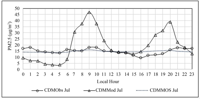
Figure 7. Concentration profiles of average hourly values of observed PM2.5, modeling, and MOS at the CDM station for the month of July 2016. There is no observed data for the month of February.

Figure 8. Concentration profiles of average hourly PM2.5 values observed, modeling, and MOS at the ATE station for the month of February 2016. There is no observed data for the month of July.
upward trend from 0:00 to 8:00 hours in the morning. Between 0:00 and 5:00 hours in the morning there is a decrease in vehicular traffic, so this increase in concentration suggests that it is the product of industrial activities and/or transport of pollutants by air, since in the Lima-East zone, 20% of the industries of Metropolitan Lima are established there [58] [61] . In addition the lack of green areas in the area allows for the resuspension of particulate material. The mean hourly values observed, predicted, and improved with the PM2.5 MOS were 24.19 ± 6.11, 27.42 ± 17.82 and 24.36 ± 0.55 μg/m3 respectively. The mean bias (MB) varied in a range of [−24.47 to 27.99 μg/m3], which indicates that the model underestimated and overestimated the observed values. Its average value was 3.24 ± 18.61 μg/m3. In other studies this value was −8.8 μg/m3 [60] , indicating that the model underestimated the measured data. The mean normalized bias (NMB) varied in a range of [−0.78 to 1.40] with an average value of 0.18 ± 0.80. In other studies this value was −0.122 (−12.2%) [60] . The mean square root (RMSE) error varied in a range of [9.86 to 40.87 μg/m3], with an average value of 23.01 ± 8.24 μg/m3. Other studies show that this parameter was 47.9 μg/m3 [60] .
For the month of February and July Figure 9 shows the hourly profiles of average PM2.5 values observed, modeled, and MOS at the SBJ station. The average statistical parameters of observed PM2.5, model and MOS in February were 14.45 ± 3.13, 4.10 ± 2.38 and 14.54 ± 0.51 μg/m3. The factor that relates PM25 Mod/PM2.5 Obs is 0.28. Therefore, the model underestimated the observed data. In other studies this relation was 1.14 [60] and 1.13 [62] . In the month of July, the aforementioned average values were 18.72 ± 3.47 and 18.90 ± 11.89 and 18.57 ± 1.63. μg/m3 respectively. In other studies, the average values observed and predicted were 30.31, 31.14 μg/m3 and 1.03 [62] respectively. In this case the model had an excellent performance. The mean bias (MB) in February varied in a range of [−17.46 to −1.95 μg/m3] with an average of −10.34 ± 5.05 μg/m3, which indicates that the model underestimated the observed data. In other studies this parameter was −8.8 μg/m3 [60] . In this case the model also underestimated the observed values. The mean bias (MB) in July varied in a range of [−14.36 to 18.08 μg/m3] with an average value of 0.18 ± 10.83 μg/m3, so the model underestimated and overestimated the observed values. In others studies this value was −25.0 μg/m3 [60] indicating that the model also underestimated the observed values. The mean normalized bias (NMB) in February varied in a range of [−0.92 to −0.23] with an average of −0.68 ± 0.24. In other studies the value was −0.054 (−5.4%) [63] .
The mean normalized bias (NMB) in July varied in a range of [−0.78 to 1.03] with an average of 0.00 ± 0.56. In other studies this value was −0.50 [59] . The RMSE in February had a range of [4.74 to 18.92 μg/m3] with an average value of 12.23 ± 4.43 μg/m3. In other studies this value was 12.68 μg/m3 [64] . While in July its range and average were [5.14 to 25.23 μg/m3] and 14.42 ± 5.55 μg/m3 respectively. In other studies this value was 55.3 μg/m3 [60] . In both months the observed data show characteristics of vehicular traffic behavior, decrease of the
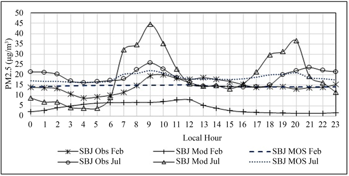
Figure 9. Concentration profiles of average hourly PM2.5 values observed, modeling, and MOS at the SBJ station for the months of February and July 2016.
concentration between 0:00 and 5:00 hours, and an increase in PM2.5 concentration between 6:00 and 9:00 hours that is when traffic activates. The model in July captures underestimated and overestimating the observed values of traffic behavior. The MOS improves the forecasts of the model in both months.
At the STA station (Figure 10) the mean hourly PM2.5 concentrations observed, predicted, and MOS were 21.78 ± 4.64, 10.62 ± 7.55 and 22.65 ± 1.04 μg/m3 respectively. Other studies show that the mean values observed and predicted were 77.8 and 69.6 μg/m3 [59] respectively. The mean bias (MB) varied in a range of [−25.09 to 2.23 μg/m3] with an average value of −11.16 ± 8.23 μg/m3 which indicates that the model underestimated the observed values. Other studies conducted in summer show that this parameter was −4.7 μg/m3 [60] which indicates that the model also underestimated the observed data. The NMB value ranged from [−0.86 (−86%) to 0.13 (13%)] with an average value of −0.51 ± 0.37. Other studies show that this parameter was 2.73%] [62] . The RMSE varied in a range of [9.10 to 26.16 μg/m3] with an average value of 15.36 ± 4.77 μg/m3. In another study this value was 8.94 μg/m3 [65] . As expected, the MOS improves the predicted values and has a better performance.
At the CRB station (Figure 11), in February, the mean hourly PM2.5 concentrations observed, predicted, and MOS were 21.51 ± 4.32, 20.44 ± 14.83 and 20.56 ± 0.04 μg/m3 respectively. The greater standard deviation of the model means that there is greater dispersion in the forecast and more uniform data in the improved forecast. The PM2.5 Mod/PM2.5 Obs factor is 0.96, and in other studies these values were 12.6, 8.6 μg/m3 and 0.68 [38] . In the month of July, these average values were of 31.53 ± 7.46, 42.69 ± 19.56 and 15.80 ± 0.92 μg/m3 respectively with a PM2.5 Mod/PM2.5 Obs factor of 1.48. Other studies show that these parameters were 30.31, 31.14 μg/m3 and 0.97 [62] respectively. The mean bias (MB) in February was maintained in a range of [−23.65 to 20.81 μg/m3] so that the model underestimated and overestimated the observed values, and its average value was −0.07 ± 17.20 μg/m3. In other studies in the summer
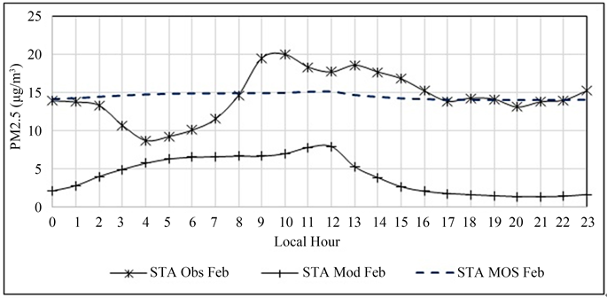
Figure 10. Concentration profiles of average hourly PM2.5 values observed, modeling, and MOS at the STA station for the month of February 2016. There is no observed data for the month of July.
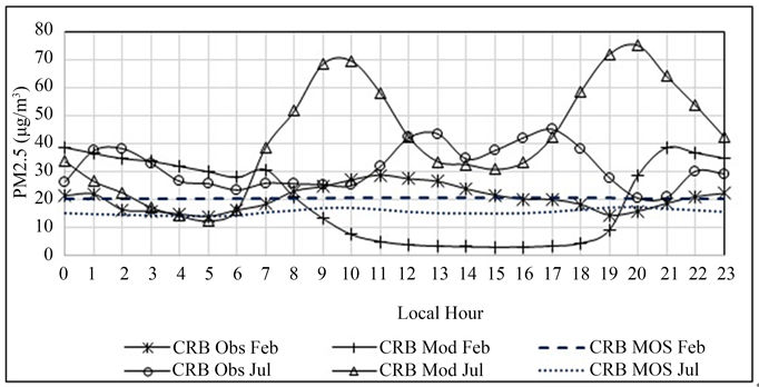
Figure 11. Concentration profiles of average hourly PM2.5 values observed, modeling, and MOS at the CRB station for the months of February and July 2016.
season this parameter was −2.0 μg/m3 [66] indicating that the model underestimated the observed average values, while the average bias (MB) in July varied in a range of [−15.43 to 55.13 μg/m3], with an average value of 11.15 ± 22.90 μg/m3, the data observed were underestimated and overestimated by the model.
In other studies the average was 5.4 μg/3 [67] indicating that the model overestimated the observed data. The NMB remained in a range of [−0.87 (−87%) to 1.18 (118%)] with an average value of 0.10 ± 0.84. In other studies the values were −8.8% (−0.088) [68] and 47% (0.47) [69] . In these cases the model underestimated and overestimated the observed values. The mean normalized bias (NMB) in July varied in a range of [−0.50 to 2.69] with an average value of −0.48 ± 0.92. In other studies, the average value was 0.04 [70] . The error of the mean square root (RMSE) in February varied in a range of [9.29 to 25.56 μg/m3], with an average value of 20.05 ± 3.90 μg/m3. In other studies the value was 47.9 μg/m3 [60] . While in July this parameter varied in a range of [13.45 to 57.56 μg/m3] with an average value of 28.80 ± 12.32 μg/m3. In other studies the average value was of 55.3 μg/m3 [60] . The data observed in July exceeded the air quality standard 20 times and in February 4 times.
At the HCH station (Figure 12) the mean hourly PM2.5 concentrations observed, predicted, and MOS in February were 14.40 ± 4.42, 18.89 ± 13.41 and 14.44 ± 0.52 μg/m3 respectively and the factor PM2.5 Mod/PM25 Obs was 0.76. The improved forecast has the lowest standard deviation, which means less dispersion. That is, a greater uniformity in the data. In studies such as that of [38] the average values observed and predicted were 12.6 and 8.6 μg/m3 with a factor of 1.47. The mean bias (MB) varied in a range of [−17.20 to 23.82 μg/m3] with an average value of 4.50 ± 14.75 μg/m3, which indicates that the model underestimated and overestimated the observed values. In other studies this parameter was 9.5 μg/m3 [71] which indicates that the model underestimated the observed data. The mean normalized NMB bias varied in a range of [−0.74 to 2.18] with an average value of −0.43 ± 1.12, and 18.8% (0.188) [71] . Mean root mean square
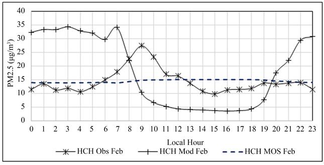
Figure 12. Concentration profiles of average hourly PM2.5 values observed, modeling, and MOS at the HCH station for the month of February 2016. There is no observed data for the month of July.
error (RMSE) varied in a range of [7.52 to 31.11 μg/m3], with an average value of 17.83 ± 8.20 μg/m3. In other studies the average value was 30.5 μg/m3 [60] .
At the PPD station (Figure 13), in February, the mean hourly PM2.5 concentrations observed, forecast, and MOS were 28.41 ± 5.05, 15.21 ± 6.20 and 28.49 ± 4.16 μg/m3 respectively with a factor PM2.5 Mod/PM2. 5 Obs of 0.54. These average values in the study of [72] were 24 and 31 μg/m3 with a factor of 1.29. The average values for July were 37.95 ± 3.47 and 35.33 ± 16.01 and 37.70 ± 0.50 μg/m3 respectively. The model shows greater dispersion than the observed data, which is graphically confirmed and by its greater standard deviation. In the cities of Beijing and Tianjin in winter, average observed and predicted data were reported of 190 and 135.71 μg/m3 [73] and 99 ± 54, 55 ± 32 μg/m3 [74] respectively. The average values observed exceeded the air quality standard in February from 7:00 hours and in July 24:00 hours. This area is urban and has massively circulating vehicles of different categories: urban, interprovincial, and heavy cargo transport.
The mean bias (MB) in February varied in a range of [−29.64 to 1.42 μg/m3] with an average value of −13.20 ± 10.70 μg/m3, which indicates that the model underestimated and overestimated the observed values. In the studies conducted by [65] and [60] the values of this parameter were −5.9173 μg/m3 and −28.9 μg/m3 respectively, in both cases the model underestimated the values observed. In July its range was from [−5.85 to 30.49 μg/m3] with an average of −2.62 ± 16.80 μg/m3, the model underestimated and overestimated the observed values. This parameter was −54.29 μg/m3 [74] and 17.7 μg/m3 [67] . In the first case, the model underestimates, and in the second case, it overestimated the observed values. The mean normalized bias (NMB) in February varied in a range of [−0.78 (78%) to 0.07 (7%)] with an average value of −0.42 (42%) ± 0.32 (32%). This parameter in the studies carried out in the summer season by [65] and [60] were −31.84% and −18.5% respectively. The mean normalized bias (NMB) in July varied in a range of [−0.68 to 0.90] with an average value of −0.06 ± 0.46,
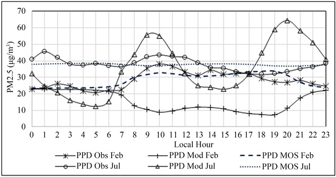
Figure 13. Concentration profiles of average hourly PM2.5 values observed, modeling, and MOS at the PPD station for the months of February and July 2016.
indicating a general error of −6%. In other studies this value was of 15.9% (0.159) [67] and 0.03 (3%) [62] . The mean square root (RMSE) error in February varied in the range of [8.28 to 31.84 μg/m3], with an average value of 19.07 ± 7.24 μg/m3. In the study conducted by [60] this parameter was 30.5 μg/m3. The error of the mean root mean square (RMSE) July varied in a range of [10.98 to 32.15 μg/m3] with an average value of 20.05 ± 6.26 μg/m3. In the study conducted by [67] the value of this parameter was 92.39 ± 0.83 μg/m3 [73] .
At the SMP station (Figure 14) the observed, predicted, and MOS average concentrations in February were 12.04 ± 2.00, 6.63 ± 4.35 and 12.50 ± 1.33 μg/m3 respectively with a PM2.5 Mod/PM2.5 Obs factor of 0.55. These average values in the [72] ’s study were 42.5 and 37.9 μg/m3 with a factor of 0.89 and 9.33, 12.23 μg/m3 with a factor of 1.31 [75] . The average values in July were of 18.34 ± 3.26, 25.60 ± 15.55 and 18.24 ± 0.14 μg/m3 respectively. In the study of [67] the values were 111.32 and 135.02 μg/m3 respectively. The mean bias (MB) in February varied in a range of [−12.30 to 6.10 μg/m3] with an average value of −5.41 ± 5.70 μg/m3, which indicates that the model underestimated and overestimated the observed values. In other studies in the summer season this parameter was 0.12 μg/m3 [76] which indicates that the model has a good performance and a slight overestimation and −4.43 μg/m3 [62] . In this case the model underestimated the observed values.
The mean bias (MB) in July varied in a range of [−3.94 to 37.75 μg/m3] with an average value of 7.26 ± 15.77 μg/m3, which indicates that the model underestimated and overestimated the observed values. Other Winter studies show that the values of this parameter were 17.7 μg/m3 [67] and −6.00 μg/m3 [72] , indicating that the model underestimated and overestimated the observed values. The mean normalized bias (NMB) in February varied in a range from [−0.83 to 0.75] with an average value of −0.40 ± 0.48. In other studies this value was 2.2% (0.022) [76] and −12.2 [60] . This parameter in July varied in a range of [−0.70 to 2.05] with an average value of 0.44 ± 0.89. In other studies this value was 0.159
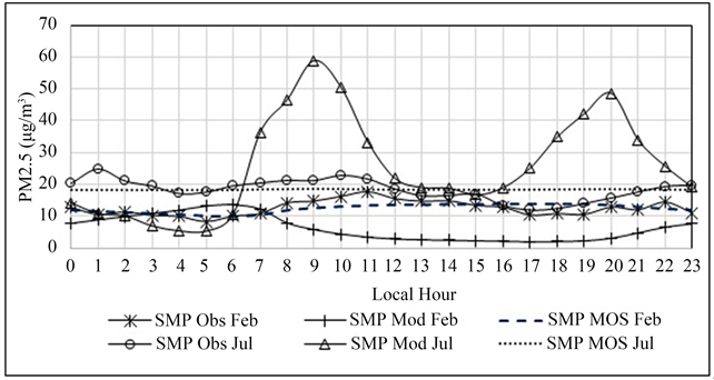
Figure 14. Concentration profiles of average hourly PM2.5 values observed, modeling, and MOS at the SMP station for the months of February and July 2016.
[67] and 0.03 [62] . The mean square root (RMSE) error in February varied in a range of [4.85 to 13.82 μg /m3], with an average value of 9.57 ± 2.56 μg/m3. In other studies in the summer season, these parameters were 47.9 μg/m3 and 0.5 [60] and 12.68 μg/m3 and 0.42 [64] . In July the range of this parameter was of [7.47 to 41.49 μg/m3] and its average of 18.45 ± 8.89 μg/m3. In other studies for the winter season the RMSE values were 55.3 μg/m3 [60] and 10.9 μg/m3 [72] .
At the VMT station (Figure 15), the average observed, forecast and MOS hourly concentrations in July were 20.02 ± 6.36, 10.39 ± 5.86 and 20.13 ± 2.45 μg/m3 respectively with a PM2.5 Mod/PM2.5 Obs factor of 0.52. At the Arese station (Italy) the values were 71.3 ± 30.7, 21.4 ± 7.65 μg/m3 respectively with a factor of 0.43 [77] . The mean bias (MB) varied in a range of [−0.90 to 3.18 μg/m3], with an average value of −9.63 ± 6.70 μg/m³. The model mostly underestimated the observed value. In other studies the average values were 17.7 μg/m3 [64] and 5.8 μg/m3 [72] . In both cases the model overestimated the observed values. The mean normalized bias (NMB) varied in a range of [−0.87 to 0.22] with an average of −0.46 ± 0.32. Other studies show that this value was 0.15 [72] , and 47% (0.47) [69] . The root mean squared error (RMSE) varied in a range of [5.14 to 29.30 μg/m3] with an average value of 15.07 ± 6.52 μg/m3. In other studies, these values were 15.4 μg/m3 and 0.61 [72] .
At the SJL station (Figure 16) the observed, predicted, and MOS average concentrations in February were 22.02 ± 4.40, 25.34 ± 17.51 and 22.08 ± 2.05 μg/m3 respectively with a PM2.5 Mod/PM2.5 Obs factor of 1.15. In the study directed by [38] these parameters were 12.6 and 8.6 μg/m3 and 0.68, and in that of [62] of 38.13, 33.70 μg/m3 and 0.88. In July, the values of this parameter were 33.67 ± 4.39, 36.36 ± 16.67, 33.31 ± 0.25 μg/m3 respectively, with a factor of 1.08. In the study directed by [64] , values were 13.73 and 11.80 μg/m3 respectively, with a factor of 0.86, and in the study of [72] , they were 42.5 and 37.9 μg/m3 with a factor of 0.89. The mean bias (MB) in February varied in a range of [−24.95 to 33.98 μg/m3], with an average value of 3.32 ± 19.51 μg/m3. The model underestimated and overestimated the observed values. In other studies the average
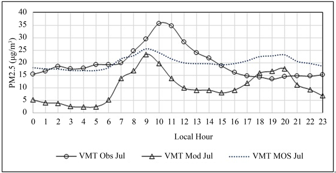
Figure 15. Concentration profiles of average hourly PM2.5 values observed, modeling, and MOS at the VMT station for the month of July 2016. There is no observed data for the month of February.
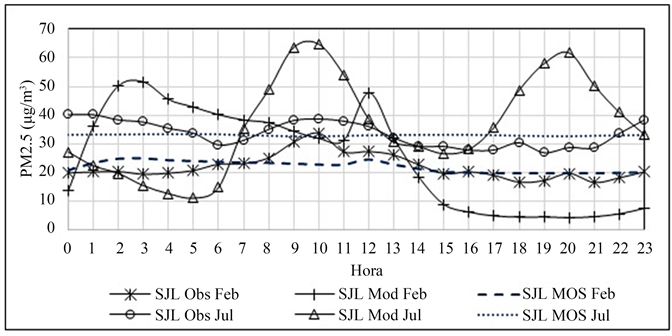
Figure 16. Concentration profiles of average hourly PM2.5 values observed, predicted, and MOS at the SJL station for the months of February and July 2016.
values in summer were −4.43 μg/m3 [62] and −1.41 μg/m3 [64] . In both cases the model overestimated the observed values. In July this parameter varied in a range of [−22.72 to 32.35 μg/m3] with an average value of 2.69 ± 17.55 μg/m3, which indicates that the model underestimated and overestimated the observed values. In other studies the values of this parameters were 17.7 μg/m3 [62] and −4.20 μg/m3 [72] . In the first case, the model overestimated, and in the second case, underestimated the observed values. The mean normalized bias (NMB) in February varied in a range of [−0.82 to 2.03] with an average value of 0.23. ± 0.20, in other summer studies this parameter was −11.6% (−0.12) [62] , −10.6% (−0.11) [59] . This parameter in July varied in a range of [−0.67 to 1.10] with an average value of 0.10 ± 0.53. In other winter studies the values of this parameter were 15.9% (0.159) [67] and −49.8% (0.498) [59] . The mean square root (RMSE) error in February ranged from [11.98 to 39.90 μg/m3] with an average value of 22.23 ± 7.37 μg/m3. In other studies, the value of this parameter was 47.9 μg/m3 [60] and 12.68 μg/m3 [64] . In July, its range was [10.41 to 38.08 μg/m3] with an average value of 23.00 ± 8.74 μg/m3. In other studies, the average values were 55.3 μg/m3 [60] and 28.8 μg/m3 [59] .
4. Conclusions
Some possible reasons why a numerical model of time underestimates or overestimates the measured concentrations of particulate matter are: 1) There is uncertainty in the emissions inventory. At this point there is a consensus, as many investigations mention it. Comparisons of emission inventories have revealed large differences in emission estimates, finding that differences for example in primary organic carbon emissions can be as high as 140% [78] , the emissions inventory can introduce errors of the order of 40 up to 70% in PM [78] . 2) The WRF/Chem, being a complex numerical model of time, requires simplifications in its parameterizations in order to evaluate the different physical and chemical parameters, and the finite difference method is the most used. Therefore, the model naturally has uncertainties. Different types of uncertainties are mentioned in [79] . 3) The biases depend on several factors such as the inventory of emissions used, the horizontal resolution, and selected parameterizations [38] [80] .
1) From the analysis of the meteorological parameters, temperature and relative humidity, the model in February and July satisfactorily simulated these parameters.
2) The average PM2.5 concentrations observed in the month of July are higher than in February, probably because the relative humidity in July 2016 was higher than the relative humidity in February 2016.
3) The standard deviations of PM2.5 concentrations observed in February are higher than in July, except for the CRB and SBJ stations, which is indicated by a greater dispersion of the observed data.
4) The standard deviations of the PM2.5 model in February are greater than those observed, generally by a factor of 2.5, indicated by a greater dispersion of model data with the exception of the SBJ station.
5) The standard deviations of the PM2.5 model in July are greater than those observed, in general by a factor of 3.2, indicated by a greater dispersion of the model data, with the exception of the VMT station.
6) In February, the air quality standard (PM2.5, 25 μg/m3) was exceeded at the PPD station and in July at the CRB, PPD, VMT and SJL stations. Living in an environment where air quality is poor, poses a risk to people’s health, and reduces life expectancy.
7) The vehicle flow in the AML decreases from 0:00 to 5:00 hours. Therefore, the concentration of the particulate PM2.5 material decreases. The average value profiles at the CDM, SBJ, STA, CRB, PPD, SMP, SJL stations (only in July) capture this behavior in both months. However, at the ATE, HCH, VMT and SJL stations (February) the trend is the increase in concentration, probably by receiving contributions from air transport.
8) From 0:00 to 5:00 hours, the PM2.5 model at CDM (overestimated), ATE (overestimated), SBJ (underestimated), STA (underestimated and overestimated), CRB (February: overestimated, July: underestimated), HCH (overestimated), PPD (February, underestimated and overestimated, July: underestimated), SMP (February: underestimated and overestimated, July: underestimated), VMT (underestimated), SBJ (February: overestimated, July, underestimated).
9) The PM2.5 model better estimates the behavior of vehicular traffic in July than in February.
10) In all cases, the concentration profiles of the values improved with MOS are close to the profiles of average values observed.
Acknowledgements
The authors would like to thank the National Service of Meteorology and Hydrology (SENAMHI) for having provided information on PM2.5 and PM10 concentrations, as well as running the WRF-Chem model, as well as the Department of Atmospheric Sciences at the Institute of Astronomy, Geophysics and Atmospheric Sciences (IAG), University of São Paulo, Brazil, as well as Carol Ordoñez Aquino for her help with making map of geographical location of SENAMHI-Lima air quality stations. We thanked the anonymous reviewer that it has given interesting suggestions to improve the article.
Conflicts of Interest
The authors declare no conflicts of interest regarding the publication of this paper.
Cite this paper
Reátegui-Romero, W., Sánchez-Ccoyllo, O.R., de Fatima Andrade, M. and Moya-Alvarez, A. (2018) PM2.5 Estimation with the WRF/Chem Model, Produced by Vehicular Flow in the Lima Metropolitan Area. Open Journal of Air Pollution, 7, 215-243. https://doi.org/10.4236/ojap.2018.73011
References
- 1. ING (2014) National Geographic Institute, Republic of Peru. Lima. http://www.ign.gob.pe
- 2. WPR (2018) World Population Review. Lima.
- 3. INEI (2012) Automotive Park in Circulation at National Level, According to Department, 2003-2012. Lima. (In Spanish)
- 4. Wei, X., Li, H., Yang, N., Wong, S., Chong, M., Shi, L., Wong, M., Xu, J., Zhang, D., Tang, J., Li, D.Q. and Mengf, G.S. (2015) Changes in the Perceived Quality of Primary Care in Shanghai and Shenzhen, China: A Difference-In-Difference Analysis. Bulletin of the World Health Organization, 93, 407-416.
- 5. Incecik, S. and Im, U. (2012) Air Pollution in Mega Cities: A Case Study of Istanbul. In Air Pollution-Monitoring, Modelling and Health, Croatia, InTech, 77-116. https://doi.org/10.5772/32040
- 6. Chang, D., Song, Y. and Liu, B. (2009) Visibility Trends in Six Megacities in China 1973-2007. Atmospheric Research, 94, 161-167. https://doi.org/10.1016/j.atmosres.2009.05.006
- 7. Gurjar, B. and Lelieveld, J. (2005) New Directions: Megacities and Global Change. Atmospheric Environment, 39, 391-393. https://doi.org/10.1016/j.atmosenv.2004.11.002
- 8. Parrish, D. and Zhu, T. (2009) Clean Air for Megacities. Science, 326, 674-675. https://doi.org/10.1126/science.1176064
- 9. Molina, M. and Molina, L. (2013) Megacities and Atmospheric Pollution. Journal of the Air & Waste Management Association, 54, 644-680.
- 10. Kim, J., Smorodinsky, S., Lipsett, M., Singer, B., Hodgson, A. and Ostro, B. (2004) Traffic Related Air Pollution near Busy Roads: East Bay Children’s Respiratory Health Study. American Journal of Respiratory and Critical Care Medicine, 170, 520-526. https://doi.org/10.1164/rccm.200403-281OC
- 11. Pérez, N., Pey, J., Cusack, M., Reche, C., Xavier, Q.X., Alastuey, A. and Viana, M. (2010) Variability of Particle Number, Black Carbon, and PM10, PM2.5, and PM1 Levels and Speciation: Influence of Road Traffic Emissions on Urban Air Quality. Aerosol Science and Technology, 44, 486-499.
- 12. Pant, P. and Harrison, R. (2013) Estimation of the Contribution of Road Traffic Emissions to Particulate Matter Concentrations from Field Measurements: A Review. Atmospheric Environment, 77, 78-97. https://doi.org/10.1016/j.atmosenv.2013.04.028
- 13. Brown, L., Collings, N., Harrison, R., Maynard, A. and Maynard, R. (2003) Ultrafine Particles in the Atmosphere. Imperial College Press, London. https://doi.org/10.1142/p287
- 14. Beekmann, M., Prévôt, A., Drewnick, F., Sciare, J., Pandis, S., Denier van der Gon, H., Crippa, M., Crippa, M., Freutel, F., Poulain, L., Ghersi, V., Rodriguez, E., Beirle, S., Zotter, P., von der Weiden, S., Bressi, M., Fountoukis, C., Petetin, H., et al. (2015) In Situ, Satellite Measurement and Model Evidence on the Dominant Regional Contribution to Fine Particulate Matter Levels in the Paris Megacity. Atmospheric. Chemistry. Physics, 15, 9577-9591. https://doi.org/10.5194/acp-15-9577-2015
- 15. Seinfeld, J. and Pandys, S. (2006) Atmospheric Chemistry and Physics Drom Air Pollution to Climate Change. Jhon Wiley & Sons, Inc., New Jersey.
- 16. Ying, T., Jian, W., Jian, G.S.W., Yu, Z., Lai, Z.P. and Yin, F. (2013) Long-Term Variation of the Levels, Compositions and Sources of Size-Resolved Particulate Matter in a Megacity in China. Science of the Total Environment, 463-464, 462-468.
- 17. Zheng, M., Cass, G., Ke, L., Wang, F., Schauer, J., Edgerton, E. and Russell, A. (2007) Source Apportionment of Daily Fine Particulate Matter at Jefferson Street, Atlanta, GA, during Summer and Winter. Journal of the Air & Waste Management Association, 57, 228-242.
- 18. Dockery, D., Pope III, C., Xu, X., Spengler, J., Ware, J., Fay, M., Ferris, B. and Speizer, F. (1993) An Association between Air Pollution and Mortality in Six U.S. Cities. Journal of Medicine, 329, 1753-1759. https://doi.org/10.1056/NEJM199312093292401
- 19. Byeong, L., Bumseok, K. and Kyuhong, L. (2014) Air Pollution Exposure and Cardiovascular Disease. Toxicological Research, 30, 71-75.
- 20. Carbajal, L., Barraza, A., Durand, R., Moreno, H., Espinoza, R., Chiarella, P. and Romieu, I. (2007) Impact of Traffic Flow on the Asthma Prevalence among School Children in Lima, Peru. Journal of Asthma, 44, 197-202. https://doi.org/10.1080/02770900701209756
- 21. IAMAT (2016) Country Health Advice (Peru). General Health Risks: Air Pollution.
- 22. Robinson, C., Baumann, L., Gilman, R., Romero, K., Combe, J., Cabrera, L., Hansel, N., Barnes, K., Gonzalvez, G., Wise, R., Breysse, P. and Checkley, W. (2018) The Peru Urban versus Rural Asthma (PURA) Study: Methods and Baseline Quality Control Data from a Cross-Sectional Investigation into the Prevalence, Severity, Genetics, Immunology and Environmental. BMJ Open, 2, e000421.
- 23. Chung, B. (2008) Control of Chemical Pollutants in Peru. Revista Peruana de Medicina Experimental y Salud Pública, 25, 413-418. (In Spanish)
- 24. Underhill, L., Bose, S., Williams, D., Romero, K., Malpartida, G., Breysse, P., Klasen, E., Combe, J., Checkley, W. and Hansel, N. (2015) Association of Roadway Proximity with Indoor Air Pollution in a Peri-Urban Community in Lima, Peru. International Journal of Environmental Research and Public Health, 12, 13466-13481. https://doi.org/10.3390/ijerph121013466
- 25. Fischer, K. (2017) Improving Sustainable Development in Lima through Public Transportation Investment. Perspectives on Business and Economics, 35, 125-134.
- 26. Minsa (2015) Esda-Environmental Performance Study 2003-2013. (In Spanish)
- 27. Gonzales, G., Zevallos, A., Gonzales, C., Nuñez, D., Carmen Gastañaga, C., Cabezas, C., Naeher, L. and Levy, K.S.K. (2014) Environmental Pollution, Climate Variability and Climate Change: A Review of Health Impacts on the Peruvian Population. Peruvian Journal of Experimental Medicine Public Health, 31, 547-556. (In Spanish)
- 28. Digesa (2011) National Environmental Health Policy. Ministry of Health, Lima. (In Spanish)
- 29. Pijnappel, A. (2011) Statistical Post Processing of Model Output from the Air Quality Model LOTOS-EUROS. Stageverslag, De Bilt.
- 30. Glahn, H. and Lowry, D. (1972) The Use of Model Output Statistics (MOS) in Objective Weather Forecasting. Journal of Meteorology, 11, 1203-1211. https://doi.org/10.1175/1520-0450(1972)011<1203:TUOMOS>2.0.CO;2
- 31. CMCL (2018) Climate in Miraflores and Climate of Lima. Lima.
- 32. T. Scientific (2007) TEOM 1405 Ambient Particulate Monitor.
- 33. T. Scientific (2018) Model 5014i Beta Instruction Manual Continuous Ambient Particulate Monitor.
- 34. Vara, A., Andrade, M., Kumar, P., Ynoue, P. and Muñoz, A. (2016) Impact of Vehicular Emissions on the Formation of Fine Particles in the Sao Paulo Metropolitan Area: A Numerical Study with the WRF-Chem Model. Atmospheric Chemistry Physics, 16, 777-797. https://doi.org/10.5194/acp-16-777-2016
- 35. Sánchez-Ccoyllo, O., Ordoñez-Aquino, C., Muñoz, A., Alan Llacza, A., Andrade, M., Liu, Y., Reátegui, W. and Brasseur, G. (2018) Modeling Study of the Particulate Matter in Lima with the WRF-Chem Model: Case Study of April 2016. International Journal of Applied Engineering Research, 13, 10129-10141.
- 36. Andrade, M., Ynoue, R., Dias, E., Todesco, E., Vara, A., Ibarra, S., Droprinchinski, L., Martins, J. and Barreto, V. (2015) Air Quality Forecasting System for Southeastern Brazil. Frontiers in Environmental Science, 3, 1-14. https://doi.org/10.3389/fenvs.2015.00009
- 37. Grell, G., Peckham, S., Schmitz, R., McKeen, S., Frost, G., Skamarock, W. and Eder, B. (2005) Fully Coupled ‘‘Online’’ Chemistry within the WRF Model. Atmospheric Environment, 39, 6957-6975.https://doi.org/10.1016/j.atmosenv.2005.04.027
- 38. Tuccella, P., Curci, G., Visconti, G., Bessagnet, B., Menut, L. and Park, P. (2012) Modeling of Gas and Aerosol with WRF/Chem over Europe: Evaluation and Sensitivity Study. Journal of Geophysical Research, 117, D03303. https://doi.org/10.1029/2011JD016302
- 39. Gupta, M. and Mohan, M. (2013) Assessment of Contribution to PM10 Concentrations from Long Range Transport of Pollutants Using WRF/Chem over a Subtropical Urban Airshed. Atmospheric Pollution Research, 4, 405-410. https://doi.org/10.5094/APR.2013.046
- 40. Skamarock, W., Klemp, J., Dudhia, J., Gill, D., Barker, D., Duda, M., Huang, X., Wang, W. and Powers, J. (2008) A Description of the Advanced Research WRF Version 3.
- 41. Peckham, S., McKeen, G.V.S., Ahmadov, R., Wong, Y., Barth, M., Pfister, G., Wiedinmyer, C., Fast, J., Gustafson, W., Ghan, S., Zaveri, R., Easter, R., Barnard, J. and Chapman, E. (2017) WRF-Chem Version 3.8.1 User’s Guide.
- 42. Tie, X., Madronich, S., Li, G., Ying, Z., Zhang, R., Garcia, A., Taylor, J. and Liu, Y. (2007) Characterizations of Chemical Oxidants in Mexico City: A Regional Chemical Dynamical Model (WRF-Chem) Study. Atmospheric Environment, 41, 1989-2008. https://doi.org/10.1016/j.atmosenv.2006.10.053
- 43. Tie, X., Geng, F., Peng, L., Gao, W. and Zhao, C. (2009) Measurement and Modeling of O3 Variability in Shanghai, China: Application of the WRF-Chem Model. Atmospheric Environment, 43, 4289-4302. https://doi.org/10.1016/j.atmosenv.2009.06.008
- 44. Chou, M. and Suarez, M. (1999) Technical Report Series on Global Modeling and Data Assimilation—A Solar Radiation Parameterization for Atmospheric Studies.
- 45. Mlawer, E.T.J., Brown, P., Iacono, M. and Clough, S. (1997) Radiative Transfer for Inhomogeneous Atmospheres: RRTM, a Validated Correlated-k Model for the Longwave. Journal of Geophysical Research, 16, 663-682.
- 46. Hong, S., Noh, Y. and Dudhia, J. (2005) A New Vertical Diffusion Package with an Explicit Treatment of Entrainment Processes. Monthly Weather Review, 134, 2318-2341.
- 47. Monin, A. and Obukhov, A. (1954) Basic Laws of Turbulent Mixing in the Surface Layer of the Atmosphere. Tr. Akad. Nauk SSSR Geophiz. Inst., 30.
- 48. Grell, G. (1991) Prognostic Evaluation of Assumptions Used by Cumulus Parameterizations. Monthly Weather Research, 121, 764-787.
- 49. Lin, Y., Farley, R. and Orville, H. (1983) Bulk Parameterization of the Snow Field in a Cloud Model. Journal of Climate and Applied Meteorology, 22, 1065-1092. 2.0.CO;2>https://doi.org/10.1175/1520-0450(1983)022<1065:BPOTSF>2.0.CO;2
- 50. Wild, O., Zhu, X. and Prather, M. (2000) Fast-J: Accurate Simulation of In- and Below-Cloud Photolysis in Tropospheric Chemical Models. Journal of Atmospheric Chemistry, 37, 245-282. https://doi.org/10.1023/A:1006415919030
- 51. Stockwell, W., Kirchner, F. and Kuhn, M. (1997) Mechanisms for Air Quality Modeling: Development and Applications of the Regional Atmospheric Chemistry Mechanism. Journal of Geophysical Research, 25, 847-879. https://doi.org/10.1029/97JD00849
- 52. Ackermanna, I., Hassa, H., Memmesheimera, M., Ebela, A., Binkowskia, F. and Shankara, U. (1998) Modal Aerosol Dynamics Model for Europe: Development and First Applications. Atmospheric Environment, 32, 2981-2999. https://doi.org/10.1016/S1352-2310(98)00006-5
- 53. Wilks, D. (2006) Statistical Methods in the Atmospheric Sciences. 2nd Edition, Academic Press, Cambridge.
- 54. Yu, S., Eder, B., Dennis, R., Chu, S. and Schwartz, S. (2006) New Unbiased Symmetric Metrics for Evaluation of Air Quality Models. Atmospheric Science Letters, 7, 26-34.
- 55. Zhang, H., Chen, G., Hu, J., Che, S., Wiedinmyer, C., Kleeman, M. and Ying, Q. (2014) Evaluation of a Seven-Year Air Quality Simulation Using the Weather Research and Forecasting (WRF)/Community Multiscale Air Quality (CMAQ) Models in the Eastern United States. Science of the Total Environment, 473-474, 275-285.
- 56. Time and Date (2016) Past Weather in Lima, Peru. Lima.
- 57. Deuman and Walsh (2005) Informe Final Estudio dE Linea Base Ambiental Cosac I. Preparado para Protransporte. Lima.
- 58. Senamhi (2013) Evaluación de la Calidad del AIRE en Lima Metropolitana. Lima.
- 59. Cai, C., Zhang, X., Wang, K., Zhang, Y., Wang, L., Zhang, Q., Duan, F., He, K. and Shao, C. (2016) Incorporation of New Particle Formation and Early Growth Treatments into WRF/Chem: Model Improvement, Evaluation, and Impacts of Anthropogenic Aerosols over East Asia. Atmospheric Environment, 124, 262-284. https://doi.org/10.1016/j.atmosenv.2015.05.046
- 60. Xu, Y., Yang, Z., Qiang, Z. and Ke, B. (2016) Application of Online-Coupled WRF/Chem-MADRID in East Asia: Model Evaluation and Climatic Effects of Anthropogenic Aerosols. Atmospheric Environment, 124, 321-336.
- 61. INEI (2014) Perú Estructura Empresarial 2013. Lima. (In Spanish)
- 62. Yin, X., Huang, Z., Zheng, J., Yuan, Z., Zhu, W., Huang, X. and Chen, D. (2017) Source Contributions to PM2.5 in Guangdong Province, China by Numerical Modeling: Results and Implications. Atmospheric Research, 186, 63-71. https://doi.org/10.1016/j.atmosres.2016.11.007
- 63. Kang, D., Mathur, R. and Rao, T. (2010) Assessment of Bias-Adjusted PM2.5 Air Quality Forecasts over the Continental United States during 2007. Geoscientific Model Development, 3, 309-320. https://doi.org/10.5194/gmd-3-309-2010
- 64. Balzarini, A., Pirovano, G., Honzak, L., Zabkar, R., Curci, G., Forkel, R., Hirtl, M., San José, R., Tuccella, P. and Grell, G. (2015) WRF-Chem Model Sensitivity to Chemical Mechanisms Choice in Reconstructing Aerosol Optical Properties. Atmospheric Environment, 115, 604-619. https://doi.org/10.1016/j.atmosenv.2014.12.033
- 65. Baró, R., Jiménez, P., Balzarini, A., Curci, G., Forkel, R., Grell, G., Hirtl, M., Honzak, L., Langer, M., Pérez, J., Pirovano, G., San José, R., Tuccella, P., Werhahn, J. and Zabkar, R. (2015) Sensitivity Analysis of the Microphysics Scheme in WRF-Chem Contributions to AQMEII Phase 2. Atmospheric Environment, 115, 620-629. https://doi.org/10.1016/j.atmosenv.2015.01.047
- 66. Wang, K., Zhang, Y., Yahya, K., Wu, S. and Grell, G. (2015) Implementation and Initial Application of New Chemistry-Aerosol Options in WRF/Chem for Simulating Secondary Organic Aerosols and Aerosol Indirect Effects for Regional Air Quality. Atmospheric Environment, 115, 716-732. https://doi.org/10.1016/j.atmosenv.2014.12.007
- 67. Li, T., Wang, H., Zhao, T., Xue, M., Wang, Y., Che, H. and Jiang, C. (2016) The Impacts of Different PBL Schemes on the Simulation of PM2.5 during Severe Haze Episodes in the Jing-Jin-Ji Region and Its Surroundings in China. Advances in Meteorology, 2016, Article ID: 6295878.
- 68. Ming, T., Yang, Z. and Daiwen, K. (2011) Application of WRF/Chem-MADRID for Real-Time Air Quality Forecasting over the Southeastern United States. Atmospheric Environment, 45, 6241-6250.
- 69. Wang, L., Zhang, Y., Wang, K., Zheng, B., Zhang, Q. and Wei, W. (2014) Application of Weather Research and Forecasting Model with Chemistry (WRF/Chem) over Northern China: Sensitivity Study, Comparative Evaluation, and Policy Implications. Atmospheric Environment, 124, 1-14.
- 70. Hu, J., Chen, J., Ying, Q. and Zhang, H. (2016) One-Year Simulation of Ozone and Particulate Matter in China Using WRF/CMAQ Modeling System. Atmospheric Chemistry and Physics, 16, 10333-10350.
- 71. Wang, L., Wei, Z., Wei, W., Fu, J., Meng, C. and Ma, S. (2015) Source Apportionment of PM2.5 in Top Polluted Cities in Hebei, China Using the CMAQ Model. Atmospheric Environment, 122, 723-736. https://doi.org/10.1016/j.atmosenv.2015.10.041
- 72. Liu, Y., Hong, Y., Fana, Q., Wang, X., Chand, P., Chena, X., Lai, A., Wang, M. and Chen, X. (2017) Source-Receptor Relationships for PM2.5 during Typical Pollution Episodes in the Pearl River Delta City Cluster, China. Science of the Total Environment, 596-597, 194-206. https://doi.org/10.1016/j.scitotenv.2017.03.255
- 73. Chen, D., Xie, X., Zhou, Y., Lang, J., Xu, T., Yang, N., Zhao, Y. and Liu, X. (2017) Performance Evaluation of the WRF-Chem Model with Different Physical Parameterization Schemes during an Extremely High PM2.5 Pollution Episode in Beijing. Aerosol and Air Quality Research, 17, 262-277. https://doi.org/10.4209/aaqr.2015.10.0610
- 74. Liu, J., Mauzerallb, D., Chena, Q., Zhang, Q., Song, Y., Peng, W., Klimonte, Z., Qiua, X., Zhanga, S., Hua, M., Linf, W., Kirk, K., Smithg, R. and Zhu, T. (2016) Air Pollutant Emissions from Chinese Households: A Major and Underappreciated Ambient Pollution Source. PNAS, 113, 7756-7761.
- 75. Menut, L., Siour, G., Mailler, S., Couvidat, F. and Bessagnet, B. (2016) Observations and Regional Modeling of Aerosol Optical Properties, Speciation and Size Distribution over Northern Africa and Western Europe. Atmospheric Chemistry Physics, 16, 12961-12982. https://doi.org/10.5194/acp-16-12961-2016
- 76. Yahya, K., Wang, K., Gudoshava, M., Glotfelty, T. and Zhang, Y. (2015) Application of WRF/Chem over North America under the AQMEII Phase 2: Part I. Comprehensive Evaluation of 2006 Simulation. Atmospheric Environment, 115, 733-755. https://doi.org/10.1016/j.atmosenv.2014.08.063
- 77. De Meij, A., Bossioli, E., Penard, C., Vinuesa, J. and Price, I. (2015) The Effect of SRTM and Corine Land Cover Data on Calculated Gas and PM10 Concentrations in WRF-Chem. Atmospheric Environment, 101, 177-193. https://doi.org/10.1016/j.atmosenv.2014.11.033
- 78. Zhong, M., Saikawa, E., Liu, Y., Naik, V., Horowitz, L., Takigawa, M., Zhao, Y., Lin, N. and Stone, E. (2016) Air Quality Modeling with WRF-Chem v3.5 in East Asia: Sensitivity to Emissions and Evaluation of Simulated Air Quality. Geoscientific Model Development, 9, 1201-1218. https://doi.org/10.5194/gmd-9-1201-2016
- 79. Barnard, J., Fast, J., Paredes, G., Arnott, W. and Laskin, A. (2010) Technical Note: Evaluation of the WRF-Chem “Aerosol Chemical to Aerosol Optical Properties” Module Using Data from the MILAGRO Campaign. Atmospheric Chemistry Physics, 10, 7325-7340. https://doi.org/10.5194/acp-10-7325-2010
- 80. Liao, J., Wang, T., Jiang, Z., Zhuang, B., Xie, M., Yin, C., Wang, X., Zhu, J., Fu, Y. and Zhang, Y. (2015) WRF/Chem Modeling of the Impacts of Urban Expansion on Regional Climate and Air Pollutants in Yangtze River Delta, China. Atmospheric Environment, 106, 204-214.