American Journal of Analytical Chemistry
Vol. 3 No. 8 (2012) , Article ID: 21912 , 4 pages DOI:10.4236/ajac.2012.38066
Analytical Expressions for Steady-State Concentrations of Substrate and Product in an Amperometric Biosensor with the Substrate Inhibition—The Adomian Decomposition Method
1Department of Mathematics, The Madura College, Madurai, India
2Department of Mathematics, V V College of Engineering, Tisaiyanvilai, India
Email: *raj_sms@rediffmail.com
Received June 12, 2012; revised July 18, 2012; accepted July 28, 2012
Keywords: Mathematical Modeling; Non-Linear Equation; Adomian Decomposition Method; Amperometric Biosensor; Reaction-Diffusion System; Substrate Inhibition
ABSTRACT
A mathematical model of an amperometric biosensor with the substrate inhibition for steady-state condition is discussed. The model is based on the system of non-stationary diffusion equation containing a non-linear term related to non-Michaelis-Menten kinetics of the enzymatic reaction. This paper presents the analytical expression of concentrations and current for all values of parameters . Here the Adomian decomposition method (ADM) is used to find the analytical expressions for substrate, product concentration and current. A comparison of the analytical approximation and numerical simulation is also presented. A good agreement between theoretical predictions and numerical results is observed.
1. Introduction
Biosensors are analytical devices which tightly combine biorecognition elements and physical transducer for detection of the target compounds. An amperometric biosensor is a device used for measuring concentration of some specific chemical or biochemical substance in a solution [1,2]. Biosensors use specific biochemical reactions catalyzed by enzymes immobilized on electrodes. Many enzymes are inhibited by their own substrates, leading to velocity curves that rise to a maximum and then descend as the substrate concentration increases.
In the literature, mathematical models have been widely used as an important tool to study and optimize the analytical characteristics of actual biosensors [3]. Practical biosensors contain a multilayer enzyme membrane [4], the model biosensors containing the exploratory monolayer membrane are widely used to study the biochemical behavior of biosensors [3,5]. Substrate inhibition is often regarded as a biochemical oddity and experimental annoyance.
This model is based on the system of non-stationary diffusion equations containing a non-linear term related to non-Michaelis-Menten kinetics of the enzyme reaction [2]. The dimensionless model of the biosensor with substrate and product inhibition has been constructed in order to decrease the number of biosensor properties. Substrate inhibition and interactions during biodegradation of pollutant mixtures is discussed by Okpokwasili et al. [6]. Multi-enzyme inhibitor system is investigated by Rangelova et al. [7]. Substrate inhibition kinetics of phenol degradation is described in Agarry et al. [8].
To the best of our knowledge, until now no rigorous analytical solution [9,10] has been reported for a steadystate substrate [11] and product concentration at the biosensor at mixed enzyme kinetics in the case of substrate inhibition [12-14]. As a result, in this paper we have arrived at an analytical expression corresponding to the concentration of substrate and product using ADM method for all values of reaction/diffusion parameters 
 .
.
2. Mathematical Formulation and Analysis of the Problems
2.1. Mathematical Formulation
During an enzyme-catalyzed reaction
 (1)
(1)
the substrate (S) binds to the enzyme (E) to form enzymesubstrate complex ES. While it is a part of this complex, the substrate is converted to product (P). The rate of the appearance of the product depends on the concentration of the substrate. The basic model used in this work and a definition of the coordinate system are shown in Figure 1. The simplest scheme of non-Michaelis-Menten kinetics, for example may be obtained by addition into MichaelisMenten scheme (Equation (1)), a stadium of the interaction of the enzyme substrate complex (ES) with another substrate molecule (S) (Equation (2)) following the generation of the non-active complex (ESS) [2]:
 (2)
(2)
The steady state non-linear differential equations for the substrate inhibition are [14]
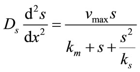 (3)
(3)
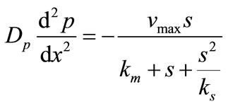 (4)
(4)
where  and
and  are the diffusion coefficient of the substrate and product within the enzyme layer. s and p are the concentration of substrate and product at any position in the enzyme layer.
  is the maximal enzymatic rate attainable when the enzyme is fully saturated with substrate,
  denotes the Michaelis-Menten constant and d is the thickness of the enzyme layer. The equation is solved for the following boundary conditions.
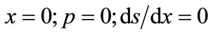 (5)
(5)
 (6)
(6)
The current density i(t) of the biosensor at time t is expressed as usual,
 (7)
(7)
We introduce the following set of dimensionless variables

 (8)
(8)
where S and P represent the dimensionless concentration of substrate and product respectively.  and denote the corresponding reaction diffusion parameters.
  represents the dimensionless distance.
  represents the saturation parameters. The governing non-linear reaction/diffusion Equations (3) and (4) are expressed in the following non-dimensionless format [14]:
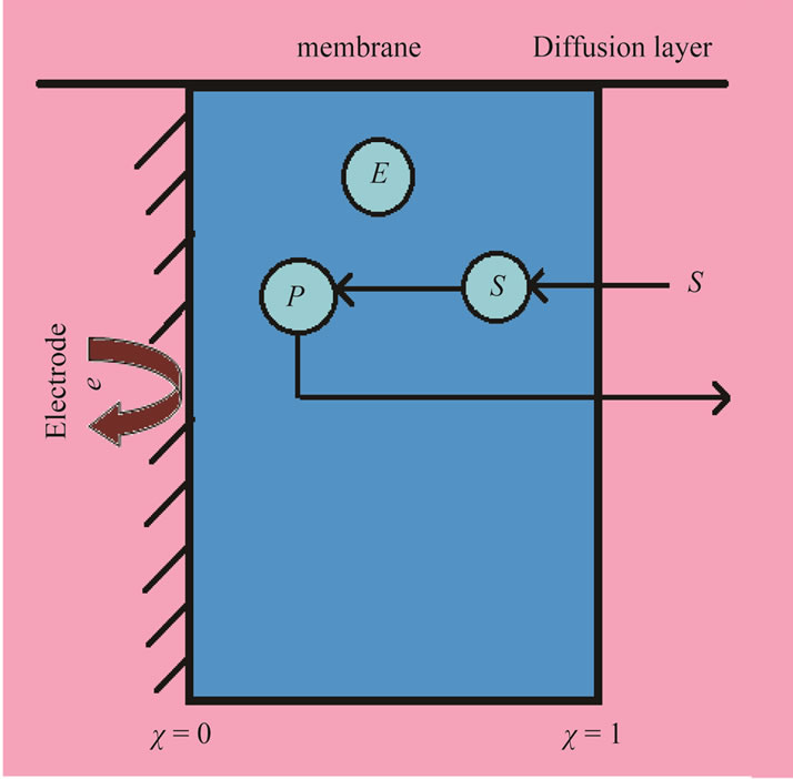
Figure 1. Schematic representation of biosensor.
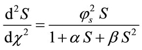 (9)
(9)
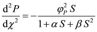 (10)
(10)
An appropriate set of boundary conditions is given by:
 (11)
(11)
 (12)
(12)
Adding Equations (9) and (10) we obtain,
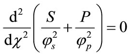 (13)
(13)
Integrating Equation (13) twice we get:
 (14)
(14)
From the above equation, we get the dimensionless concentration of product in terms of concentration of substrate as follows:
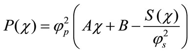 (15)
(15)
The constants A and B can be obtained using the boundary conditions given by the Equations (11) and (12). The substrate and product concentrations are all related processes. The dimensionless current is given by
 (16)
(16)
3. Concentrations of Substrate and Product under Steady-State Condition
3.1. Analytical Solution Using ADM
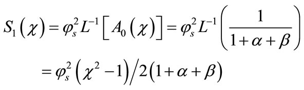
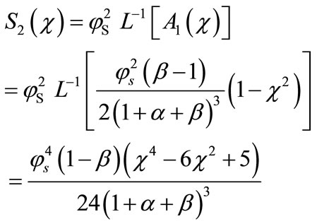
In this paper, the Adomian decomposition method (see Appendix A) is used to solve non-linear differential equations. The ADM [15-19] yields, without linearization, perturbation or transformation, an analytical solution in terms of a rapidly convergent infinite power series with easily computable terms. The analytical expression of concentration (see Appendix B) of the substrate is as follows:
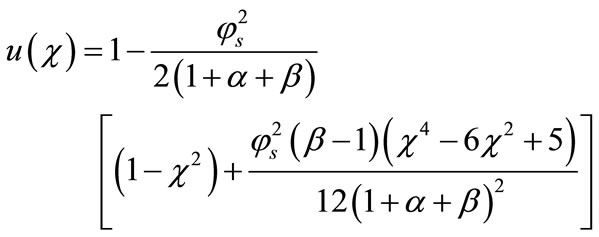 (17)
(17)
From this result and the boundary conditions (11) and (12) we can obtain the value of the constant A and B as follows:

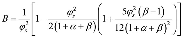
Now the product’s concentration  can be obtained from the Equation (15).
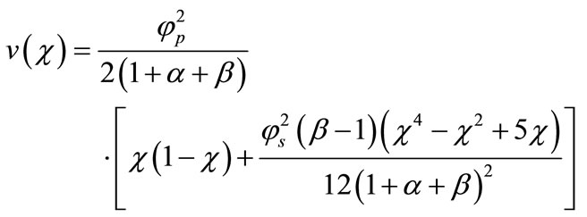 (18)
(18)
We get the dimensionless current,
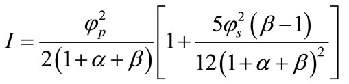 (19)
(19)
3.2. Numerical Simulation
The non-linear reaction/diffusion equations (Equations (9) and (10)) for the boundary conditions (Equations (11) and (12)) are also solved numerically. We have used the function pdex4 in Scilab/Matlab numerical software, to solve the initial-boundary value problems for parabolicelliptic partial differential equations numerically. Its numerical solution is compared with the analytical results obtained using ADM method.
4. Results and Discussion
Equations (17) and (18) represent the closest and simplest form of approximate analytical expressions for the normalized concentration of substrate and product for all values of parameters . Equation (19) represents the new approximate analytical expression of current. The numerical solution is compared with the analytical results in Figures 2-5. Figures 2-4 present the analytical and numerical concentration profiles of substrate for all values of parameters
 . The concentration of substrate and product depend upon Thiele module and saturation parameters. The Thiele module
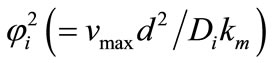 , essentially compares the rate of enzyme reaction (
 ) and diffusion in the enzyme layer (
 ).
).
We observe the rise and downfall of concentration profiles in two cases. 1) If Thiele modulus is small ( ), then enzyme kinetics predominate in the biosensor response. The overall kinetics is governed by the total amount of active enzyme; 2) The response is under diffusion control, if the Thiele module is large (
 ), which is observed at high catalytic activity and active membrane thickness or at low reaction rate constant
  or diffusion coefficient values
 .
.
Figure 2 illustrates the concentration profiles of substrate S for various values of reaction diffusion parameter of substrate . The concentration of the substrate decreases with the increasing values of
 .
.
From Figures 3 and 4 we infer that the concentration profiles of substrate S increases with the increasing values of saturation parameters .
.
The concentration profiles of the product P are compared with the numerical results in Figure 5, illustrating the concentration profiles of the product P for various
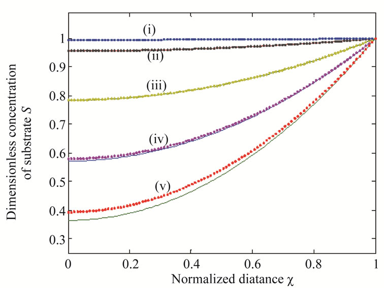
Figure 2. Dimensionless concentration of substrate S (Equation (17)) versus normalized distance χ for α = 10, β = 0.5 and for various values of . (i)
. (i) ; (ii)
 ; (iii)
 ; (iv)
 ; (v)
; (v) . Solid lines represent the analytical solution whereas the dotted lines for the numerical solution.
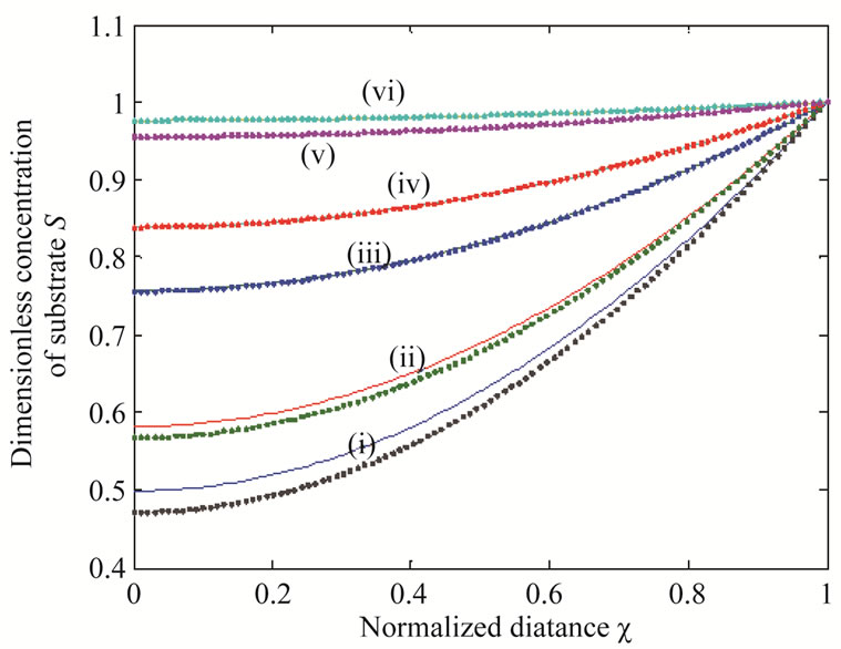
Figure 3. Dimensionless concentration of substrate S (Equation (17)) versus normalized distance χ for β = 0.5,  and for various values of α. (i) α = 0.1; (ii) α = 1; (iii) α = 5; (iv) α = 10; (v) α = 50; (vi) α = 100. Solid lines represent the analytical solution whereas the dotted lines for the numerical solution.
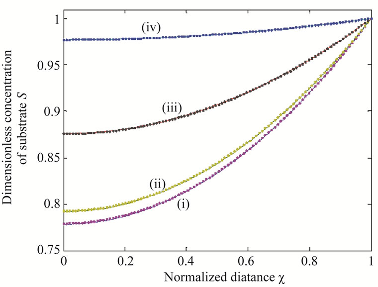
Figure 4. Dimensionless concentration of substrate S (Equation (17)) versus normalized distance χ for α = 10,  and for various values of β. (i) β = 0.1; (ii) β = 1; (iii) β = 10; (iv) β = 100. Solid lines represent the analytical solution whereas the dotted lines for the numerical solution.
values of . In all the cases the concentration of the product P increases with the increasing value of parameter
 . Figure 6 shows the dimensionless concentration of substrate S (Equation (17)) and product P (Equation (18)) versus normalized distance
  for some fixed values of parameters (
 ,
, and
and ). From Figure 6, it is inferred that the concentration of the substrate S increases and attains its maximum value 1 at
 . The concentration of the product P increases within the enzyme matrix from both the interfaces (
 and
and ) and reaching a maximum value at the middle of the membrane which is determined
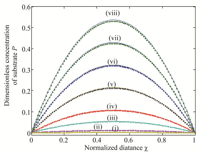
Figure 5. Dimensionless concentration of product P (Equation (18)) versus normalized distance χ for α = 10, β = 0.5,  and for various values of
 . (i)
. (i) ; (ii)
 ; (iii)
 ; (iv)
 ; (v)
; (v) ; (vi)
 ; (vii)
 ; (viii)
 . Solid lines represent the analytical solution whereas the dotted lines for the numerical solution.

Figure 6. Dimensionless concentration of substrate S (Equation (17)) and product P (Equation (18)) versus normalized distance χ for α = 10, β = 0.5,  and
and .
.
by the kinetics of the enzyme reaction and diffusion properties of the reactants.
Determination of Current
The parameter of greatest interest in an amperometric biosensor is the current, which is related to the flux of electroactive material to the electrode surface. The variation in current versus saturation parameters  are shown in Figures 7 and 8 respectively. It is evident from the figures that the current I (Equation (19)) increases when
  or
or  increases or thickness of the mem-

Figure 7. Variation of normalized current I (Equation (19)) against α for the fixed values of , β = 5 and various values of
 . (i)
. (i)  = 1; (ii)
  = 10; (iii)
  = 50; (iv)
  = 100.
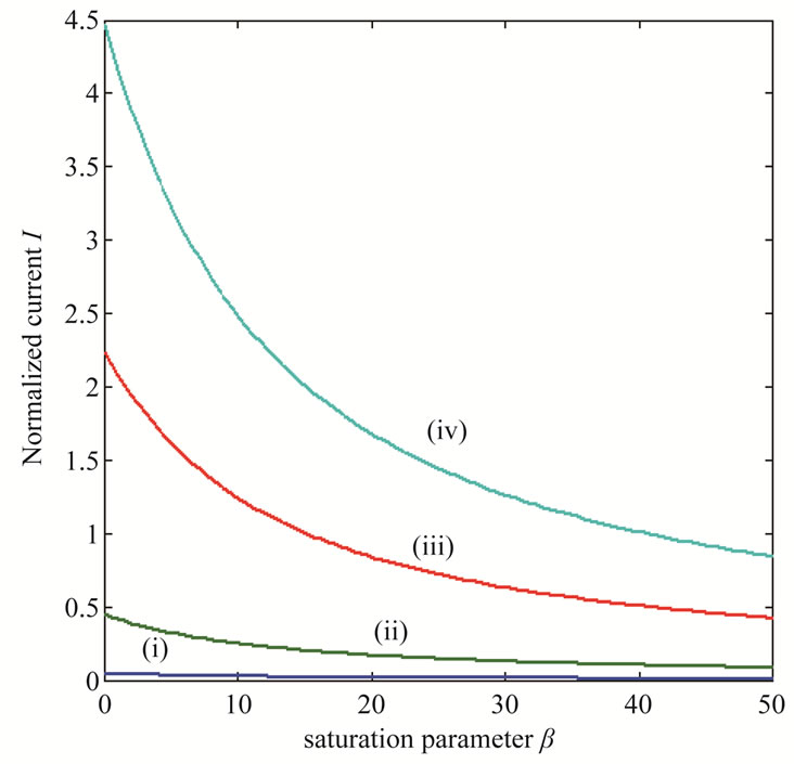
Figure 8. Variation of normalized current I (Equation (19)) against β for the fixed values of , α = 10 and various values of
 . (i)
. (i)  = 1; (ii)
 ; (iii)
 ; (iv)
  = 100.
brane d increases. Furthermore, when  is greater than 10, all the curves reach the steady state value for all values of
 . When
  is greater than 50, all the curves reach the steady state value for various values of
 .
.
5. Conclusion
The modeling of the amperometric biosensor with the substrate inhibition is discussed. The system of non-linear differential equation has been solved using ADM method. The primary result of this work is the first accurate calculation of substrate and product concentration for all values of considered parameters, this being in good agreement with simulation results. The influence of Thiele module and active membrane thickness is also investigated. The obtained analytical results will be useful in sensor design, optimization and prediction of the electrode response. Using these results, the action of biosensor is analyzed at critical concentration of substrate and enzyme activity. Theoretical results obtained in this paper can also be used to analyze the effect of different parameters such as active membrane thickness and saturation parameters.
6. Acknowledgements
This work was supported by the Council of Scientific Industrial Research (CSIR No.: 01(2442)/10/EMR-II), Government of India. The authors also thank Mr. M.S. Meenakshisundaram, Secretary, The Madura College Board, Dr. R. Murali, The Principal, The Madura College, Madurai, Tamilnadu, India for their constant encouragement.
REFERENCES
- P. Manimozhi, A. Subbiah and L. Rajendran, “Solution of Steady-State Substrate Concentration in the Action of Biosensor Response at Mixed Enzyme Kinetics,” Sensors and Actuators B: Chemical, Vol. 147, 2010, pp. 290-297. doi:10.1016/j.snb.2010.03.008
- J. Kulys and R. Baronas, “Modeling of Amperometric Biosensors in the Case of Substrate Inhibition,” Sensors, Vol. 6, No. 11, 2006, pp. 1513-1522. doi:10.3390/s6111513
- T. Schulmeister and D. Pfeiffer, “Mathematical Modeling of Amperometric Enzyme Electrodes with Perforated Membranes,” Biosensors and Bioelectronics, Vol. 8, No. 2, 1993, pp. 75-79. doi:10.1016/0956-5663(93)80055-T
- A. J. Baeumner, C. Jones, C. Y. Wong and A. Price, “A Generic Sandwich-Type Biosensor with Nanomolar Detection Limits,” Analytical and Bioanalytical Chemistry, Vol. 378, No. 6, 2004, pp. 1587-1593. doi:10.1007/s00216-003-2466-0
- R. Baronas, F. Ivanauska and J. Kulys, “The Influence of the Enzyme Membrane Thickness on the Response of Amperometric Biosensors,” Sensors, Vol. 3, No. 7, 2003, pp. 248-262. doi:10.3390/s30700248
- G. C. Okpokwasili and C. O. Nweke, “Microbial Growth and Substrate Utilization Kinetics,” African Journal of Biotechnology, Vol. 5, No. 4, 2005, pp. 305-317.
- V. Rangelova, A. Pandelova and N. Stoiyanov, “Acta Technica Corvinensis,” Bulletin of Engineering Tome IV, 2011.
- S. E. Agarry, T. O. K. Audu and B. O. Solomon, “Substrate Inhibition Kinetics of Phenol Degradation by Pseudomonas Fluorescence from Steady State and Wash-Out Data,” Internation Journal of Environmental Science and Technology, Vol. 6, No. 3, 2009, pp. 443-450.
- A. Eswari, S. Usha and L. Rajendran, “Approximate Solution of Non-linear Reaction Diffusion Equations in Homogeneous Processes Coupled to Electrode Reactions for CE Mechanism at a Spherical Electrode,” American Journal of Analytical Chemistry, Vol. 2, 2011, pp. 93-103. doi:10.4236/ajac.2011.22010
- S. Anitha, A. Subbiah and L. Rajendran, “Approximate Analytical Solution of Nonlinear Reaction’s Diffusion Equation at Conducting Polymer Ultramicroelectrodes,” ISRN Physical Chemistry, Vol. 2012, 2012, Article ID: 745616. doi:10.5402/2012/745616
- M. V. Putz, “On the Reducible Character of HaldaneRadić Enzyme Kinetics to Conventional and Logistic Michaelis-Menten Models,” Molecules, Vol. 16, No. 4, 2011, pp. 3128-3145. doi:10.3390/molecules16043128
- M. C. Reed, A. Lieb and H. F. Nijhout, “The Biological Significance of Substrate Inhibition: A Mechanism with Diverse Functions,” Bioessays, Vol. 32, No. 5, 2010, pp. 422-429. doi:10.1002/bies.200900167
- J. Kulys, “Biosensor Response at Mixed Enzyme Kinetics and External Diffusion Limitation in Case of Substrate Inhibition,” Nonlinear Analysis: Modelling and Control, Vol. 11, No. 4, 2006, pp. 385–392.
- R. Baronas, F. Ivanauskas and J. Kulys, “Mathematical Modeling of Biosensors An Introduction for Chemists and Mathematicians,” Springer Series on Chemical Sensors and Biosensors, Vol. 9, 2010, p. 104 doi:10.1007/978-90-481-3243-0
- M. A. Mohamed, “Comparison Differential Transformation Technique with Adomian Decomposition Method for Dispersive Long-Wave Equations in (2+1)-Dimensions,” Applications and Applied Mathematics, Vol. 5, No. 1, 2010, pp. 148-166.
- O. K. Jaradat, “Adomian Decomposition Method for Solving Abelian Differential Equations,” Journal of Applied Sciences, Vol. 8, No. 10, 2008, pp. 1962-1966. doi:10.3923/jas.2008.1962.1966
- A. M. Siddiqui, M. Hameed, B. M. Siddiqui and Q. K. Ghori, “Use of Adomian Decomposition Method in the Study of Parallel Plate Flow of a Third Grade Fluid,” Communications in Nonlinear Science and Numerical Simulation, Vol. 15, No. 9, 2010, pp. 2388-2399. doi:10.1016/j.cnsns.2009.05.073
- A. Majid Wazwaz and A. Gorguis, “An Analytic Study of Fisher’s Equation by Using Adomian Decomposition Method,” Applied Mathematics and Computation, Vol. 154, No. 3, 2004, pp. 609-620. doi:10.1016/S0096-3003(03)00738-0
- H. Jafari and V. Daftardar-Gejji, “Solving Linear and Nonlinear Fractional Diffusion and Wave Equations by Adomian Decomposition,” Applied Mathematics and Computation, Vol. 180, No. 2, 2006, pp. 488-497. doi:10.1016/j.amc.2005.12.031
- N. H. Sweilam and M. M. Khader, “Approximate Solutions to the Nonlinear Vibrations of Multiwalled Carbon Nanotubes Using Adomian Decomposition Method,” Applied Mathematics and Computation, Vol. 217, No. 2, 2010, pp. 495-505. doi:10.1016/j.amc.2010.05.082
- G. Adomian, “Solving the Mathematical Models of Neurosciences and Medicine,” Mathematics and Computers in Simulation, Vol. 40, No. 1-2, 1995, pp. 107-114. doi:10.1016/0378-4754(95)00021-8
- O. D. Makinde, “Adomian Decomposition Approach to a SIR Epidemic Model with Constant Vaccination Strategy,” Applied Mathematics and Computation, Vol. 184, No. 2, 2007, pp. 842-848. doi:10.1016/j.amc.2006.06.074
- S. Loghambal and L. Rajendran, “Analytical Expressions for Steady-State Concentrations of Substrate, Oxidized and Reduced Mediator in an Amperometric Biosensor,” Kinetics and Catalysis, in press.
Appendix A
Basic Concept of the Adomian Decomposition Method (ADM)
Adomian decomposition method [18-21] depends on decomposing the non-linear differential equation
 (A.1)
(A.1)
in two components
 (A.2)
(A.2)
where L and N are the linear and the non-linear parts of F respectively. The operator L is assumed to be an invertible operator. Solving for  leads to
 (A.3)
(A.3)
Applying the inverse operator L on both sides of Equation (A.3) yields
 (A.4)
(A.4)
where  is a function that satisfies the condition
 . Now assuming that the solution y can be represented as infinite series of the form,
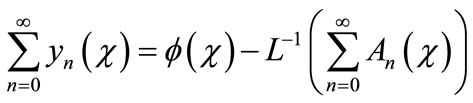 (A.5)
(A.5)
where
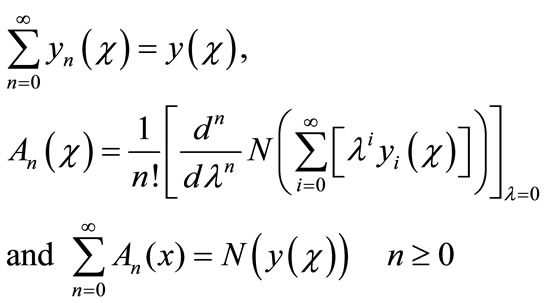 (A.6)
(A.6)
Then equating the like terms in the linear system of Equation (A.5) gives the recurrent relation
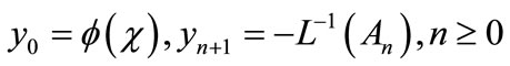 (A.7)
(A.7)
However, in practice all the terms of series in Equation (A.5) cannot be determined, and the solution is approximated by the truncated series .
.
Appendix B
Analytical Expression of Concentrations of Substrate Using the Adomian Decomposition Method
To solve the non linear Equation (9) using the Adomian decomposition method [18-23], we write the Equation (9) in the operator form,
 (B.1)
(B.1)
where
 (B.2)
(B.2)
Applying the inverse operator  on both sides of Equation (B.1) yields
 (B.3)
(B.3)
According to the ADM, the solution  can be elegantly computed by using the recurrence relation (A.7). Using this relation we obtain,
 (B.4)
(B.4)
where A and B are constants of integration. Using the boundary condition Equation (9) we get,
 (B.5)
(B.5)
 (B.6)
(B.6)
 are the Adomian polynomials of
 . We can find the first few Adomian polynomial coefficients
  using Equation (A.6) as follows:
 (B.7)
(B.7)
 (B.8)
(B.8)
The remaining polynomials  can be generated easily, using Equation (A.6). Applying the following boundary conditions
 (B.9)
(B.9)
Using Equation (B.6) we can obtain the following results:
 (B.10)
 (B.11)
Adding Equations (B.5), (B.10) and (B.11), we get the concentration of substrate (Equation (17)) as in the text.
Appendix C
Scilab/Matlab Program for the Numerical Solution of Non-Linear Equations (9) and (10)
function pdex4
m = 0;
x = [0 0.00002 0.00004 0.00006 0.00008 0.00010];
t = [0 2 4 6 8 10];
sol = pdepe(m,@pdex4pde,@pdex4ic,@pdex4bc,x,t);
u1 = sol(:,:,1);
u2 = sol(:,:,2);
u3 = sol(:,:,3);
figure
plot(x,u1(end,:))
title('Solution at t = 2')
xlabel('Distance x')
ylabel('u1(x,2)')
figure
plot(x,u2(end,:))
title('Solution at t = 2')
xlabel('Distance x')
ylabel('u2(x,2)')
% -------------------------------------------------------------
function [c,f,s] = pdex4pde(x,t,u,DuDx)
s0=1;
Ds=10^(-10);
v=10^(-2);
d=10^(-4);
ks=0.001;
km=0.01;
c = [1;1];
f = [1; 1] .* DuDx;
F1 =v*u(1)/(km+u(1)*(1*u(1)/ks));
s =[-F1; F1];
% -------------------------------------------------------------
function u0 = pdex4ic(x);
u0 = [1; 0];
% -------------------------------------------------------------
function [pl,ql,pr,qr] = pdex4bc(xl,ul,xr,ur,t)
pl = [0; ul(1)];
ql = [1; 0];
pr = [ur(1)-1; ur(2)];
qr = [0; 0];
NOTES
*Corresponding author.