1. Introduction
Over the past several years, different enzyme reactions governed by different equations have been identified in the field of biochemistry. Estimation of kinetic parameters of these enzyme reactions is one of the important problems [1] -[4] . The nonlinearity in the functional expression for the reaction rate, in terms of substrate concentration and other parameters, makes the parameter estimation problem difficult. Graphical techniques such as Lineweaver-Burk’s method and the use of Dixon plot to estimate parameters [5] -[7] were in vogue for some time. These methods rely on linearizing the Michaelis-Menten equation in the case of simple enzyme reactions. For complex enzyme reactions, such techniques do not furnish reliable results. This has prompted Wilkinson to propose non-linear regression for the estimation of enzyme parameters [8] . Using Wilkinson non-linear regression coupled with a modified Fibonacci search method, Atkins outlined a computer program for fitting the Hill equation directly to experimental data [9] . Following this, numerous software packages have been developed [10] -[11] to perform parameter estimation interactively. Most of these packages have fixed menus and do not allow the user to incorporate possible changes to the underlying algorithm.
The goal of this article is to explain the nonlinear regression technique briefly and show four simulation examples of enzyme reactions. The programming is done in MATLAB, a registered trade mark of MathWorks, Inc. MATLAB is a high-level language and interactive environment that enables one to perform computationally intensive tasks faster than with traditional programming languages. The syntax of various functions in MATLAB makes implementing difficult, mathematical steps very straightforward.
Today, use of MATLAB has almost become a de facto standard among engineers and computer scientists both in academia and industry. Faculty and students of biochemistry can easily learn this software using numerous tutorials available on-line or introductory books such as [18] -[21] . Further, it is easy for biologists to develop interaction with other engineers and scientists in the language of MATLAB. In this paper we shall discuss the basic principle behind nonlinear regression, and supplement it with simulation examples1.
2. Parameter Estimation via Nonlinear Regression
One of the challenges faced in a biochemistry laboratory while studying enzyme kinetics is to decide comprehensive levels of the substrate concentration. For example, it is hard to determine the maximum concentration, minimum concentration, and to know how best to space the intermediate levels and so on. In practice, one may have to plot the data and go through a few iterations before endorsing the data for further processing. After satisfactory acquisition of the data, which invariably carries measurement inaccuracies, enzyme parameters appearing in the governing model can be estimated using the non-linear regression technique.
Let us consider a functional relationship that expresses the reaction rate v in terms of the independent variable(s) and some parameters. For example, in the case of a simple enzyme-substrate uninhibited reaction it is given by the Michaelis-Menten equation:
 . (1)
. (1)
In Equation (1) above, the substrate concentration s is the independent variable, and  and
and  are enzyme parameters representing the maximum reaction velocity and the Michaelis constant respectively. Numerically,
  equals s when
 . In general, there may be more independent variables than s alone, which for convenience, could be put in a vector of N elements say,
 . Let the vector
  denote a set of P parameters. Here the superscript T denotes the transpose. This generalization would become clearer after three more examples that are discussed in this paper. The dependence of v on x and β is denoted by
 . Let
. Let  stand for the mth data sample. The subscript m in all occurrences except in the Michaelis constant
  indicates the mth observation. Since measurements are subject to experimental errors, we shall write:
 (2)
(2)
where the measurement error,  , is assumed to be a normally distributed random variable with a mean zero and a variance of
 . Given a set of measured values of Equation (2), the parameter estimation problem involves finding an estimate of β that reduces a measure of error, usually the sum of weighted (with the weights wm) residual squares WRSS, denoted by
 :
:
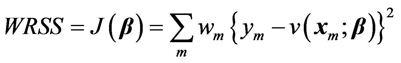 . (3)
. (3)
Our objective is to minimize  with respect to β. It is hard to find the minimum of
  by explicitly differentiating and solving for global minimum. Iterative methods are usually employed. Nonlinear regression is a convenient technique [8] [22] that allows us to estimate the unknown parameters by linearizing Equation (2) at each iteration starting from an initial guess
 . This is done by first expressing
  with the first two terms in its Taylor’s series expansion around an estimate, initially taken as
 . Then the mth element in Equation (2) can be written as:
 (4)
(4)
here  is assumed to be a small increment in the parameter vector. This can be done for all the observations m = 1 to M.
Now treating the vector  as the residual
  at 0th iteration, we can write:
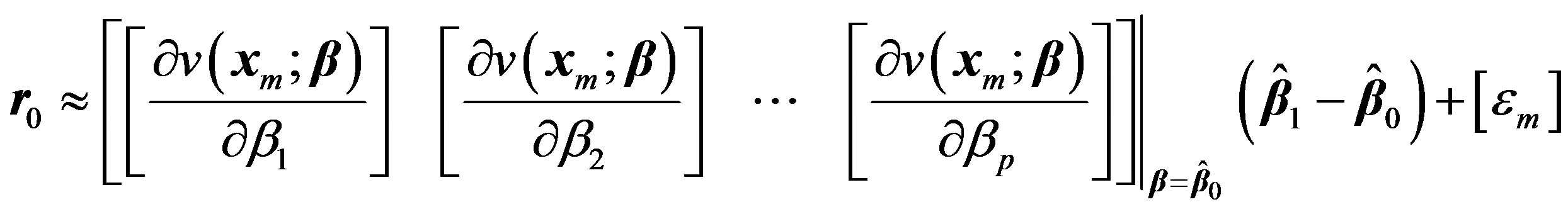 (5)
(5)
This process can be iterated by replacing 0 and 1 with k and k + 1 respectively. Denoting the matrix involving the derivatives in Equation (5) at kth iteration by Gk we get,
 . (6)
. (6)
The weighted least squares solution for this can be written in terms of generalized inverse of Gk [23] [24] as:
 (7)
(7)
where
 (8)
(8)
is the covariance matrix of .
.
Equation (7) helps in estimating the parameters of a given model recursively; but is in a generalized form. For the enzyme researchers or students to be able to code this in MATLAB, they need to understand each symbol in (7) and how to express the same for a given model. In the next section four types of enzyme models are considered and expressions for various elements of ,
, , and
, and  are given as they relate to each model. In Appendix I, MATLAB code is provided for Example III. For other examples, the same code could be edited with minimum effort by replacing the expressions of these vectors/matrices appropriately and could be executed. With this idea in mind, in the next section, Equation (7) is specialized for four different models.
3. Four Models
3.1. Model I: A Simple Uninhibited Enzyme Substrate Reaction
Let us first consider the case of a simple uninhibited enzyme substrate reaction. As mentioned earlier in the paper, s denotes the concentration of the substrate, Vmax the maximum reaction velocity, and Km the Michaelis constant, which equals the substrate concentration at half the maximum rate.
Governing equation (Michaelis-Menten equation):
 (9)
(9)
Variables and parameters:
 (10)
(10)
The mth element of the residue:
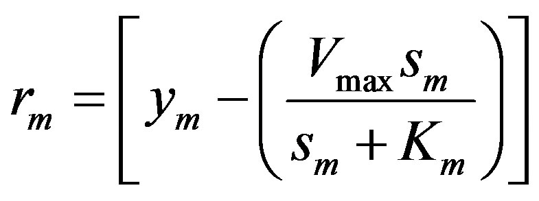 (11)
(11)
Elements of the mth row of  matrix:
 (12)
(12)
3.2. Model II: Competitive Inhibitor Enzyme Substrate Reactions
With other symbols remaining the same as in Model I, let i denote the concentration of inhibitor. The competitive reaction is governed by the Michaelis-Menten equation:
 (13)
(13)
Variables and parameters:
 (14)
(14)
The mth element of the residue:
 (15)
(15)
Elements of the mth row of  matrix:
 (16)
(16)
In passing, it might be mentioned that if the data points are collected for various inhibitor values, one could vectorize them into a single column. Accordingly, the value for i in Equation (16) should be substituted.
3.3. Model III: Allosteric Monosubstrate Enzyme
For our third model, the allosteric enzyme reaction is considered. This is governed by the Hill equation involving an empirical parameter n.
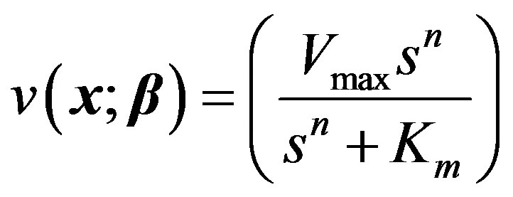 (17)
(17)
Variables and parameters:
 (18)
(18)
The mth element of the residue:
 (19)
(19)
Elements of the mth row of  matrix:
 (20)
(20)
3.4 Model IV: Allosteric Enzyme with Two Species of Ligand Sites
This is governed by two Hill equations combined as:
 (21)
(21)
Variables and parameters:
 (22)
(22)
The mth element of the residue:
 (23)
(23)
The six elements of the mth row of  matrix:
 (24)
(24)
In the next section four simulation examples are given based on the preceding four models.
4. Simulation Examples
4.1 Example I―Simple Uninhibited Reaction
Data consisting of 10 samples are simulated in case of a hypothetical enzyme with Km = 240 nM and Vmax = 80 mmol/min/mg substrate using MATLAB. A zero mean unit variance random number with Gaussian density is added as measurement error. The substrate and the reaction rate are shown in Table 1. We shall take ∑ as a 10 × 10 unit matrix. Thus, WRSS can be called RSS.
The parameters estimated using the program written in MATLAB are:
 ,
,  , and the RSS = 0.142. Figure 1 shows the enzyme reaction rate versus substrate concentration in the units specified in Table 1. In order to render a better visualization, we have provided the relief of the error surface defined in Equation (2) with unity weights in Figure 2(a). Also, Figure 2(b) shows the contours of the same plot. Note that the contours are ever widening ellipses with the global minimum shown by an asterisk. Also plotted in this figure is the learning trajectory obtained by joining all the estimated parameters over 6 iterations, starting from a provisional guess of Km(0) = 20 and Vmax(0) = 25.
This simulation is repeated using the software Prism 5, a registered trademark of GraphPad, as well as the EXCEL template called anemona published in [12] . It was assuring to find that the parameters estimated were identical viz.,  , and
, and .
.

Table 1. Simulated data consisting of 10 samples in case of a hypothetical enzyme with Km = 240 nM and Vmax = 80 mmol/min/mg substrate for enzyme reaction model I.

Figure 1. Reaction rate curve for Model I. The circles are simulated measurements, solid line is the theoretical curve, stars show the model using the estimated parameters.
 (a)
(a) (b)
(b)
Figure 2. (a) Showing the relief of the error J(β) as a function of the parameters.(b) Showing the contours of the error J(β) as a function of the parameters. The global minimum is shown by an asterisk. Also shown is the learning trajectory.
4.2. Example II―Enzyme Competitive Inhibitor Case
As a second example, the data found in the GraphPad user manual [14] is used. It is reproduced in Table 2 for convenience. The parameters for this data as given by Prism 5 are:
 .
.
The parameters estimated by using MATLAB program via non-linear regression are:
 .
.
Figure 3 shows the plot of reaction curves.
A visual display of the surface of the cost function J is not possible as it is now a function of three variables: Vmax, Km and Ki. So an attempt is made to visualize this optimization problem in two steps. First, we note that when i = 0, Model II degenerates to Model I; as such, Km and Vmax are found using the data of the first and second columns of Table 2. Secondly, using these parameters in the remaining data, J is plotted in Figure 4. The global minimum is found at Ki = 2.75 in conformity with the method of non-linear regression. In MATLAB, the min command obtains minimum of a given vector. Further, it may be pointed out that the modified Fibonacci search method used by Atkins in [9] also readily finds application to accomplish this.
4.3. Example III―pNPP Hydrolysis by Alkaline Phosphatase (Hill Equation)
Determination of kinetic parameters for the hydrolysis of p-nitrophenylphosphate (pNPP) by alkaline phosphatase was reported in [17] using a program called SigrafW. Figures 5(a), (b) show the familiar structure of pNPP and AP. For convenience, the data points of Table 1 in [17] are reproduced in Table 3 and are used in this example. The parameters obtained by SigrafW, and those obtained through MATLAB simulations, as well as Prism 5 of GraphPad, are shown in Table 4.
This exercise has been attempted using anemona reported in [12] , but this tool has yielded absurd results. Both the MATLAB program and Prism are found to yield identical values for the parameters.
Using MATLAB we find that RSS is less and correlation is better. Figure 6 shows the reaction rate curves using both the results. We note that the curve obtained using the parameters reported in [17] does not pass through the observations as accurately as reported therein. The MATLAB script file for this representative example is given in Appendix I. Modifying the code for other examples is straightforward as mentioned earlier.
4.4 Example IV―ATP Hydrolysis by Alkaline Phosphatase (Sum of Two Hill Equations)
Again we take the data available in [17] for the ATP hydrolysis by alkaline phosphatase. This reaction is characterized by the sum of two Hill equations. Figure 5(c) depicts the ATP structure. The measured data is found
Table 2. Data for competitive enzyme reaction (Model II) taken from the GraphPad user manual [14] . Here i denotes the concentration of inhibitor.