Three Dimensional Numerical Modeling of Flow and Pollutant Transport in a Flooding Area of 2008 US Midwest Flood ()
1. Introduction
The Midwestern United States is one of four US geographic regions, consisting of 12 states in the United States: Illinois, Indiana, Iowa, Kansas, Michigan, Minnesota, Missouri, Nebraska, North Dakota, Ohio, South Dakota, and Wisconsin. This region has a long history of flooding, with major floods occurring several times over the recent century including 1927, 1961, 1993, 2008, and 2011. Minor flooding is a regular occurrence.
Due to a long term precipitation from December 2007 to June 2008, the Midwest had experienced one of the most wettest winter and spring, causing the soil to become so saturated that additional rainfall could quickly became runoff. In June 2008, much of the Midwestern portions received over 300 mm of rainfall as several storm systems sequentially impacted the region. The vast majority of the precipitation across the region was channeled directly into the lakes, rivers, and streams as runoff, resulting in stream flows reaching historic heights across the Midwest, particularly in many areas of Iowa, southern Wisconsin, and northern Illinois [1,2].
Huge flooding events were reported along the Mississippi River and its tributaries. A number of rivers overflowed for several weeks at a time and levees breached in numerous locations. Historical record high stream flows occurred in some of the major regional rivers including the Des Moines, Cedar and Wisconsin Rivers. Reported river crests exceeded 500-year levels in some locations. It was reported that about twenty-two levees were breached forcing evacuations and causing extensive damage by June 20, 2008. Several states, including Illinois, Indiana, Iowa, Michigan, Minnesota, Missouri, and Wisconsin, were affected by the flooding events. Navigation along the Mississippi River was affected with several of the lock and dam structures closed. The flood left two dozen people killed, 148 injured, approximately 35,000 - 40,000 people evacuated from homes and the damage region-wide was estimated to be in the tens of billions of dollars [1].
A levee of the Iowa River near Mississippi River failed in the evening of June 14, and the water in Iowa River completely flooded the town of Oakville, and thousands of acres of farmland were under water. Since the flooded water was controlled by the levees of Iowa River, Mississippi River, and a hilly area of the Mississippi Valley, an inundation zone was formed for several weeks [3,4]. As there was no outlet, after the water rose to the highest level, it kept for several days. It was observed that some pollutants, such as sewage, pig farm waste, diesel fuel and farm chemicals were leaked and transported in the water [5]. To study the transportation of the pollutant, the inundation zone was treated as a natural lake.
Due to the lack of field measured data, numerical modeling is one of the most effective approaches to study the pollutant transport processes in the flooding zone. Some well-established models, such as ECOMSED developed by Hydroqual, EFDC and WASP developed by the US Environmental Protection Agency (USEPA), CEQUAL-ICM developed by the US Army Corp of Engineers (USACE), have been used by many researchers to study the flow, water quality and pollutant transport in natural water bodies [6-9]. Dortch et al. [10] applied the CH3D-WES hydrodynamic model, originally developed by USACE, to simulate the flow field and pollutant transport of Lake Pontchartrain due to the large amount of contaminated floodwater induced by Hurricane Katrina being pumped into the lake.
A three dimensional numerical model, CCHE3D, has been developed by the National Center for Computational Hydroscience and Engineering (NCCHE) to simulate the flow and sediment transport in natural water bodies [11]. In this study, a 3D model was developed based on CCHE3D to simulate the flow fields and pollutant transport in the Oakville flood inundation zone. After the flooding wave propagation due to the levee breaching, water level rose to the highest position. The water movement in the inundation zone was mainly driven by the wind and the wind-induced flow was the major force for the pollutant transport. This study presents the validation and application of a 3D numerical model for simulating the wind-driven flow and associated pollutant transport in the flooding area of Oakville during the Midwest Flood. Remote sensing techniques using different satellite imagery acquired during the flood event were used to provide some important information, including topography of study area, locations and dimensions of building and farming facilities, and traces of pollutants on the water surface, etc., for the model’s inputs and validation.
2. Model Description
CCHE3D is a finite-element-based unsteady three-dimensional (3D) free surface turbulence model that can be used to simulate turbulent flows with irregular boundaries and free surfaces. This model is based on the 3D Reynolds-averaged Navier-Stokes equations. By applying the Boussinesq assumption, the turbulent stresses are approximated by the eddy viscosity and the strains of the flow. There are several turbulence closure schemes available including: parabolic eddy viscosity model, mixing length model, k-e model and nonlinear k-e model. This model has been verified against analytical methods and experimental data representing a range of hydrodynamics phenomena [11].
To study the wind-driven flow in the Oakville inundation zone, a parabolic vertical distribution of eddy viscosity was specified to analyze the wind-induced flow. A mass transport model was developed based on CCHE3D hydrodynamic model. The pollutant transport equation was solved using finite element method which was consistent with the numerical method employed in the CCHE3D model.
2.1. Governing Equations
The governing equations of continuity and momentum of the three-dimensional unsteady hydrodynamic model can be written as follows:
 (1)
(1)
 (2)
(2)
where ui (i = 1, 2, 3) are the Reynolds-averaged flow velocities (u, v, w) in Cartesian coordinate system (x, y, z); t is the time; r is the water density; p is the pressure; n is the fluid kinematic viscosity;  is the Reynolds stress; and fi are the body force terms.
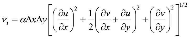
The turbulence Reynolds stresses in Equation (2) are approximated according to the Bousinesq’s assumption. These stresses are related to the mean velocity gradients and the eddy viscosity coefficients. The horizontal eddy viscosity coefficient is computed using the Smagorinsky scheme [12]:
 (3)
(3)
where Dx and Dy are the grid lengths in x and y directions, respectively. The parameter a ranges from 0.01 to 0.5.
For wind-driven flow, the vertical eddy viscosity is mainly determined by the wind stresses. Several formulas were presented to calculate the wind-induced eddy viscosity (Section 2.2).
The free surface elevation (hs) is computed using the following equation:
 (4)
(4)
where us, vs and ws are the surface velocities in x, y and z directions; hs is the water surface elevation.
The pollutant transport equation can be expressed by:
 (5)
(5)
in which u, v, w are the water velocity components in x, y and z directions, respectively; ws is the settling/floating velocity; C is the pollutant concentration in water column; Dx, Dy and Dz are the diffusion coefficients in x, y and z directions, respectively;  is the effective source term.
2.2. Wind-Induced Eddy Viscosity
In a natural lake or the Oakville flood inundation zone, wind stress is the important driving force for flow circulation. For simulating the wind driven flow, the distribution of vertical eddy viscosity is required. A parabolic eddy viscosity distribution was proposed by Tsanis [13] based on the assumption of a double logarithmic velocity profile. The eddy viscosity was expressed as:
 (6)
(6)
in which l is the numerical parameter; zb and zs are the characteristic lengths determined at bottom and surface, respectively; u*s is the surface shear velocity; H is the water depth. To use this formula, three parameters, l, zb and zs have to be specified. For some real cases with very small water depths, it may cause some problems using this formula to calculate eddy viscosity.
Koutitas and O’Connor [14] proposed two formulas to calculate the eddy viscosity based on a one-equation turbulence model. Their formulas were:
 (7)
(7)
 (8)
(8)
where
 (9)
(9)
in which, l is the numerical parameter; hz is the nondimensional elevation, .
.
In this study, a new formula was proposed to calculate the wind-induced eddy viscosity based on experimental measurements conducted in a laboratory flume with steady-state wind driven flow reported by Koutitas and O’Connor [14]. The vertical distribution of eddy viscosity was measured and used to fit a calculation formula.
In the proposed formula, the form of eddy viscosity was similar to Koutitas and O’Connor’s assumption (Equations (7) and (8)) and expressed as:
 (10)
(10)
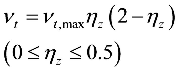
Based on measured data, a formula was obtained to calculate the vertical eddy viscosity:
 (11)
(11)
Figure 1 compares the vertical distributions of eddy viscosity obtained from experimental measurements and formulas provided by Tsanis (Equation (6)), Koutitas (Equations (7) and (8)), and the proposed formula (Equation (11)). The proposed formula can be used to calculate the eddy viscosity over the full range of water depth. At water surface ( ), Equations (6) and (8) show the eddy viscosity is zero or very closed to zero. The newly proposed formula shows due to the effect of wind shear, the eddy viscosity at the water surface is about 16% of the maximum eddy viscosity
 . This formula was used to calculate the vertical eddy viscosity in this study.
2.3. Boundary Conditions
Wind stress is generally the dominant driving force for flow currents in natural lakes. The wind shear stresses at the free surface are expressed by
 (12)
(12)
 (13)
(13)
where  is the air density; Uwind and Vwind are the wind velocity components at 10 m elevation in x and y directions, respectively. Although the drag coefficient Cd may vary with wind speed [14,15], for simplicity, many researchers assumed the drag coefficient was a constant on

Figure 1. Comparison of vertical eddy viscosity formulas and experimental data.
the order of 10−3 [16,17]. In this model, Cd was set to 0.001, and this value is applicable for simulating the wind driven flow in several natural lakes [18,19].
On the free surface, the normal gradient of pollutant concentration was set to be equal to zero. In the vicinity of the solid walls and bed, the gradients of flow properties were steep due to wall effects. The normal gradient of concentration on the wall was set to be zero.
There are many dry areas in the flooded zone, which represent the buildings of farmer facilities and islands, and wet and dry technique was applied to those areas. In the model, non-slip and the zero normal gradients boundary conditions were set for simulating the flow velocity and pollutant concentration, respectively.
2.4. Numerical Solution
The numerical model was developed based on the finite element method. Each element is a hexahedral with three levels of nine-node quadrilaterals, and the governing equations are discretized using a 27-node hexahedral (Figure 2).
Staggered grid is adopted in the model. The grid system in the horizontal plane is a structured conformal mesh generated on the boundary of the computational domain. In vertical direction, either uniform or non-uniform mesh lines are employed. In order to get more accurate results, the non-uniform mesh lines are placed with finer resolution near the wall, bed and free surface.
The unsteady equations are solved using the time marching scheme. A second-order upwinding scheme is adopted to eliminate oscillations due to advection. In this model, a convective interpolation function is used for this purpose. This function is obtained by solving a linear and steady convection-diffusion equation analytically over a one-dimensional local element shown in Figure 2. Although there are several other upwinding schemes, such as the first order upwinding, the second order upwinding and Quick scheme, the convective interpolation function is selected in this model due to its simplicity for the implicit time marching scheme [11].

Figure 2. Coordinate system and computational element (in the figure, x , h and z are axes of a local system).
The velocity correction method is applied to solve the dynamic pressure and enforce mass conservation. Provisional velocities are solved first without the pressure term, and the final solution of the velocity is obtained by correcting the provisional velocities with the pressure solution [11]. The system of the algebraic equations is solved using the Strongly Implicit Procedure (SIP) method.
Flow fields, including water elevation, horizontal and vertical velocity components, and eddy viscosity parameters were computed by CCHE3D. After getting the effective source terms SS, the pollutant concentration distribution can be simulated by solving pollutant transport Equation (5) numerically.
3. Model Validation and Verification
3.1. Model Validation for Wind-Driven Flow
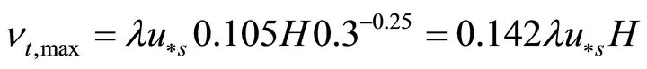
A laboratory test case was carried out in a wind-wave flume by Koutitas and O’Connor [14] to study the winddriven flow. The length and width of the measuring flume were 5 m and 0.2 m, and the water depth was 0.31 m. The vertical current profile near the middle section was measured. The developed numerical model was applied to simulate the velocity profile of the wind driven flow for the experimental case. A non-uniform grid with 21 vertical nodes with fine resolution near surface and bed were used for model validation. In the numerical modeling, both Equations (6) and (11) were used for calculating the eddy viscosity, and the simulated vertical velocity profiles were compared with experimental measurements (Figure 3). Numerical results are generally in good agreement with experimental measurements. Near the water surface, the model underestimated the velocity using Tsanis’s formula (Equation (6)) to calculate the eddy viscosity; while it overestimated the velocity by us-
Figure 3. Normalized vertical velocity profile (us = surface velocity).
ing the proposed formula (Equation (11)). Near the bottom, the simulation obtained by using the proposed formula gave better predictions.
3.2. Model Verification for the Mass Transport
The proposed numerical model was tested against an analytical solution for predicting the concentrations of a non-conservative substance in a hypothetical one-dimensional river flow with constant depth and velocity. At the middle of the river, there is a point source with constant concentration (Figure 4). Under this condition, the concentration of the substance throughout the river can be expressed as:
 (14)
(14)
where U is the velocity; C is the substance concentration; Dx is the dispersion coefficient; x is the displacement from point O; and K is the decay rate. An analytical solution given by Thomann and Mueller [20] is:
 (15)
(15)
 (16)
(16)
where C0 is the concentration at O point. In this test case, it was assumed, the water depth is 10 m and Dx is 30 m2/s, the values of K are 0, 1.0/day and 2.0/day, respectively, Figure 5 shows the concentration distributions obtained by the numerical model and analytical solution. The maximum error between the numerical result and analytical solution is less than 2%.
4. Application to Oakville Flood Zone Due to 2008 US Midwest Flood
4.1. Study Area
Due to a long period of heavy precipitation, a 500-year flood occurred in June 2008 and affected portions of the Midwest United States. In the evening of June 14, a levee

Figure 4. Test river for model verification.

Figure 5. Concentration distribution of non-conservative substance in the test river.
along the Iowa River just upstream of Oakville failed, and the water in the river rushed through the broken levee and completely flooded the small town. Figure 6 shows the flood zone and the location of the levee breaching. As the flooding area was governed by river levees and hilly area, an inundation area was formed and the high water level in this zone tented to remain for several weeks. It was reported that the length of the damaged levee was about 1100 m, and it was not completely fixed until July 1 [2,3,21]. It was estimated from the high water mark, the high water level was about 2.5 meter above the ground [22,23]. It was also observed that some oily pollutants were leaked and transported on the water surface [5]. To study the pollutant transport in the inundation zone, this flooding area can be treated as a natural lake. As this area is relatively flat, the wind is the major driving force of the water flow. To demonstrate the capabilities of the developed model, it was applied to simulate the wind-induced flow and pollutant transport.
Figure 7 shows the computational domain and topography obtained from 30 m resolution of USGS Digital Elevation Model (DEM). The inundation zone was an enclosed water body with the north-south axis spanning about 16 km, while the shorter east-west axis was about 8 km. There were many residential houses and farm facilities in this flooding zone, which could affect the flow fields. In the numerical model, they were represented with a number of dry nodes. The computational mesh was generated using the CCHE Mesh Generator. In the horizontal plane, the computational domain was represented by a 199 × 300 irregular quadrilateral mesh. In the vertical direction, it was divided into 8 non-uniform layers and mesh lines conformed to the curved and irregular bed bathymetry. The vertical distribution of the non-uniform grid was generated using the flexible and powerful two-direction stretching function with finer spacing near the surface and bottom [24].