Segmentation and Classification of Individual Clouds in Images Captured with Horizon-Aimed Cameras for Nowcasting of Solar Irradiance Absorption

Bruno Juncklaus Martins^1*, Juliana Marian Arrais¹, Allan Cerentini¹, Aldo von Wangenheim¹, Gilberto Perello Ricci Neto¹, Sylvio Mantelli²

¹PPGCC-INE, UFSC Federal University of Santa Catarina, Florianopolis, Brazil.
²FOTOVOLTAICA, INPE Brazilian National Institute for Space Research, Sao Paulo, Brazil.

DOI: 10.4236/ajcc.2023.124027                

Abstract

One important aspect of solar energy generation especially in inter-tropical sites is the local variability of clouds. Satellite images do not have temporal resolution enough to nowcast its impacts on solar plants, this monitoring is made by local cameras. However, cloud detection and monitoring are not trivial due to cloud shape dynamics, the camera is a linear and self-adjusting device, with fish-eye lenses generating a flat image that distorts images near the horizon. The present work focuses on cloud identification to predict its effects on solar plants that are distinct for every site’s climatology and geography. We used RASPBERY-PI-based cameras pointed at the horizon to allow observation of clouds’ vertical distribution, not possible with a unique fish-eye lens. A large number of cloud image identification analyses led the researchers to use deep learning methods such as U-net, HRnet, and Detectron. We use transfer learning with weights trained over the “2012 ILSVRC ImageNet” data set and architecture configurations like Resnet, Efficient, and Detectron2. While cloud identification proved a difficult task, we achieved the best results by using Jaccard Coefficient as a validation metric, with the best model being a U-net with Resnet18 using 486 × 648 resolution. This model had an average IoU of 0.6, indicating a satisfactory performance in cloud segmentation. We also observed that the data imbalance affected the overall performance of all models, with the tree class creating a favorable bias. The HRNet model, which works with different resolutions, showed promising results with a more refined segmentation at the pixel level, but it was not necessary to detect the most predominant clouds in the sky. We are currently working on balancing the dataset and mapping out data augmentation transformations for our next experiments. Our ultimate goal is to use such models to predict cloud motion and forecast the impact it will have on solar power generation. The present work has contributed to a better understanding of what techniques work best for cloud identification and paves the way for future studies on the development of a better overall cloud classification model.

Keywords

Segmentation, Cloud, Nowcasting

1. Introduction

The presence of clouds has a major effect on the photovoltaic power plants, causing significant variability in solar energy that reaches the surface, and as a consequence, in the power energy generation (Hu & Stamnes, 2000) . The detection of clouds and the estimation of their impacts on solar plants is a challenging task. Clouds are always in continuous metamorphosis. The logarithmic scale of its luminosity (Mantelli, von Wangenheim, Pereira, & Sobieranki, 2020) , the variety and dynamic of their shapes, along with their forming and extinction processes are always associated with local geography and current weather conditions. Different types of clouds and altitudes, also have distinct effects on the scattering, reflection, and absorption of solar energy, influencing energy power production. Different thicknesses, shapes, and volumes of clouds, could cause sudden changes in sky coverage trapping and releasing long and short waves resulting in significant changes in radiation throughout the day.

The World Meteorological Organization (WMO) classifies clouds by their shape, clustering, and height of their base. According to WMO¹ clouds can also be divided by groups into specific categories such as species, variety, and additional supplementary features, as described in WMO Cloud Atlas². The estimation of cloud type and coverage is made by a synoptic operator. The development of automated systems and methods of observation is still an open subject. Especially in terms of the replacement of the highly developed perception of a human observer classification.

There are commercial automated solutions available for cloud identification, in order to assess their impact on energy generation like Whole Sky Imager (WSI) (Juncklaus Martins, Cerentini, Neto, & von Wangenheim, 2021, 2022a) . This system can be configured to use single or double fish-eye surface cameras. They use pixel value analysis, and stereo techniques to evaluate the clouds. The single system poses a problem when dealing with images used for nowcasting. WSI images show in detail only clouds that lie on the zenith position. Near the horizon and close to the lens border, clouds seem to be compressed and the image degrades in the details. Double fish-eye images are coupled with additional geometric and stereo technology to determine cloud-based. But the embedded software and additional cameras are expensive and they have to be placed kilometers apart. One important feature of cloud classification is its vertical distribution in different layers. The pixel value analysis used is still far from achieving the classification proposed by WMO (Mantelli et al., 2020) .

It is desirable to estimate cloud shade casting in detail, especially when it causes a partial coverage of large power plants. Scattered cloud’s condition throughout the day has intermittent effects on the generation and does not cause only attenuation in energy. But also a surplus is known as over-irradiation by multiple reflections that result in levels of irradiance above the top of atmosphere values (Martins, Mantelli, & Rüther, 2022) . This excess could result in some operational problems with inverters, unbalanced energy generation among module strings, overloads, and even safety shutdowns (do Nascimento, Braga, Campos, Naspolini, & Rüther, 2020 ; do Nascimento, de Souza Viana, Campos, & Rüther, 2019) . Therefore, it is important to have tools to model and predict the energy generated by photovoltaic technologies (Tarrojam, Mueller, Eichman, & Samuelsen, 2012) , especially when associated with storage systems. Many energy grids combine power from multiple sources. Predicting solar power output, using accurate cloud forecasting, helps grid managers decide when to tap into alternative energy sources like wind or hydropower, ensuring a steady power supply to consumers. Additionally, precise prediction of cloud patterns allows power plants to anticipate and adjust for these variations, ensuring more consistent power output. Consistent and predictable power generation can lead to stable financial returns, since power plants can face penalties or reduced rates if they fail to deliver the promised power output to the grid. Accurate forecasting through cloud segmentation can help in avoiding such scenarios.

From the computer vision point of view, clouds could be segmented and their pathways monitored by tracking. Their impact on energy generation is measured by determining the present solar position combined with the geometric estimation of clouds shading over the power plant. There are several segmentation methods used in the classification of clouds. Mostly based on their shapes and inner features like texture, color similarity, brightness, and contour continuity in an image (Piccardi, 2004; Souza-Echer, Pereira, Bins, & Andrade, 2006; Long, Sabburg, Calbo, & Page, 2006; Mantelli, von Wangenhein, Pereira, & Comunello, 2010; Mejia et al., 2016) . The albedo of a cloud has inherent characteristics that are distinguished from common objects and outdoor scene features. Its reflectivity in the visible spectrum is higher than the other wavelengths and its luminance values are usually cropped due to camera scale limitations (Mantelli et al., 2020) . In general, objects only reflect the local surrounding radiation and this approach does not comprehensively describe albedo features and scenery under the sun. Therefore, the use of the brightness parameter is not accurate enough to distinguish a cloud. Cloud textures are random and their diffuse edges contain gray level jumps which are more similar to a phase step in large areas. To a certain degree, smaller parts of clouds are similar to the whole, and the cloud cluster has a certain fractal similarity (Li, Dong, Xiao, & Xu, 2015) . The shape, size, formation, extinction, and changing level are variable along the cloud’s pathway which made it difficult to monitor their surface shades.

Some computer vision-based methods rely on cross-classification and divide clouds into broader physical forms. These classifications are based on the shared properties of clouds, such as opacity, structure, and formation processes. Specifically, following the classification proposed by (Barrett & Grant, 1976) , clouds can be categorized as follows:

1) Stratiform, grouping Cirrostratus, Altostratus, Stratus, and Nimbostratus.

2) Cirriform, which only includes Cirrus.

3) Stratocumuliform, encompassing Cirrocumulus, Altocumulus, and Stratocumulus.

4) Cumuliform, containing only Cumulus.

5) Cumulonimbusform, exclusive to Cumulonimbus.

These groupings were chosen to explore the broader categories, understanding that there may be variations within each group. Our study aims to provide foundational insights into these groupings, which can later be refined to address specific cloud types in detail. However, due to the rare presence of Cumulonimbusform clouds in the region, we chose to exclude this category from the created dataset.

As mentioned before, the identification and classification of clouds near the horizon and the prediction of their path toward a photovoltaic installation is still an open research field. We believe that other configurations of methods combined with the camera as well as real data-oriented by machine learning could also be explored. Machine learning has gained some ground in recent years when it comes to solar irradiation prediction (Juncklaus Martins et al., 2021; Juncklaus Martins, et al., 2022a; Kumari & Toshniwal, 2021) . This is due to the popularization and easy access to artificial intelligence frameworks, which have several ready-to-use models for image segmentation and detection. There are several recent reviews on this subject made by (Juncklaus Martins et al., 2021; Kumari & Toshniwal, 2021; Mellit & Kalogirou, 2008; Pelland, Remund, Kleissl, Oozeki, & De Brabandere, 2013; Voyant et al., 2017) describing recent methods recently used, but they’re no comparative evaluation of performance among them.

In light of the aforementioned challenges and gaps in the current cloud classification and irradiation prediction methodologies, this work aims to explore existing methodologies for cloud segmentation and evaluate their performance. Our goal is to find a reliable way to classify cloud types. With these experiments we can evaluate the techniques and assess if it’s feasible to automate this process with a machine learning approach. We start by presenting previous works found in the literature related to the proposed topic. After realizing that the fish-eye lens does not provide a good indication of vertical distributions of cloud layers, we developed two systems based on Raspberry PI model 2 with the same imaging quality as WSI, pointing to the predominant direction of local clouds, with the assistance of local meteorologists (Monteiro, 2001) . We use real image data sets and check the performance of several frameworks to evaluate their performance on cloud classification. In the Materials and Methods section, we give a detailed description of used data sets production, and how our experiments were performed. In the Results section, we present and discuss briefly the achieved results. In the Discussion section, we discuss the problems faced during our experiments and make some suggestions to improve the results, and in the conclusion describe the best methods to implement the proposed task. In section 7, we present the next steps we mapped out for future experiments, given what we learned throughout the development of this work.

2. Related Works

Several machine learning techniques have been used to forecast solar irradiance in the past years (Voyant et al., 2017; Kumari & Toshniwal, 2021; Martins et al., 2022) . Some perform cloud identification by doing a binary image segmentation on either a patch of the sky or using Whole Sky Images (WSI). Others use the physical properties of clouds and the interaction with light and atmosphere while others use current meteorological data or exogenous data (Voyant et al., 2017) from side stations.

Machine learning techniques can be classified as Support Vectors, K-means, Artificial Neural Networks (ANN), and Convolutional Neural Networks. For example, in (Paletta & Lasenby, 2020) , the dataset used in this study originated from the SIRTA laboratory Haeffelin et al. (2005) , France. The RGB images were collected over a period of seven months from March 2018 to September 2018, with a resolution of 768 × 1024 pixels. The work is composed of two distinct networks merged into one which outputs the irradiance estimate. On one side, a ResNet Convolutional Neural Network (CNN) is used to extract features from sky images and on the other side, an Artificial Neural Network (ANN) treats available auxiliary data (past irradiance measurements, the angular position of the sun, etc). Both outputs are fed into another ANN, which integrates them to give its prediction.

In (Anagnostos et al., 2019) , sky images are retrieved every 10 s from sunrise to sunset with a camera equipped with a fisheye lens and 1920 × 1920 pixels resolution. Specific image features are computed for each image, then provided as inputs for the machine learning applications. The sky imaging software determines for each image the predominant sky or cloud type as one of seven categories: Cumulus (Cu); Cirrostratus (Cs), Cirrus (Ci); Cirrocumulus (Cc), Altocumulus (Ac); Clear sky (Clear); Stratocumulus (Sc); Stratus (St), Altostratus (As); Nimbostratus (Ns), Cumulonimbus (Cb). The Support Vector Classification (SVC) has been chosen with best classification results, achieving an accuracy of more than 99% of correct classifications.

The authors in (Fabel et al., 2022) focus on the semantic segmentation of ground-based all-sky images (ASIs) to provide high-resolution cloud coverage information of distinct cloud types. The authors propose a self-supervised learning approach that leverages a large amount of data for training, thereby increasing the model’s performance. They use about 300,000 ASIs in two different pretext tasks for pretraining. One task focuses on image reconstruction, while the other is based on the DeepCluster model, an iterative procedure of clustering and classifying the neural network output. The model achieved 85.75% pixel accuracy on average, compared to 78.34% for random initialization and 82.05% for pretrained ImageNet initialization. The improvement was even more significant when considering precision, recall, and Intersection over Union (IoU) of the respective cloud classes, where the improvement ranged between 5 and 20 percentage points, depending on the class. Furthermore, when compared to a Clear-sky Library (CSL) from the literature for binary segmentation, their model outperformed the CSL, reaching a pixel accuracy of 95.15%.

The study of (Ye, Cao, Xiao, & Yang, 2019) discusses the challenges of fine-grained cloud detection in different regions with varying air qualities. The authors collected WSIs from Hangzhou and Lijiang. The differences in these regions add complexity to the cloud detection problem. The authors tested their proposed method for fine-grained cloud detection and recognition against a well-known semantic segmentation model, Fully-convolutional Network (FCN). They fine-tuned a pre-trained FCN model with 400 images from their dataset, which included images from Lijiang and Hangzhou and used 8 cloud types and the sky as ground truth label classes. The results showed that their approach outperformed the FCN model. The computed evaluations were presented as the commonly used in semantic segmentation tasks, such as precision, recall, IoU for each class, and accuracy for each image. The authors achieved an average precision of 42.75%, average recall of 44.78%, average IoU 34.06% and an accuracy of 71.28%.

3. Methods

This section provides a detailed description of the dataset utilized, the image capturing methodology, and the deep learning models employed in our experiments. We differentiate our experiments into two distinct categories: Semantic and Instance Segmentation.

The experiments presented in this paper are an extension and refinement of prior empirical studies conducted by our team. Previously, we evaluated various machine learning models on the same dataset, but the classification was predicated on cloud base height. In this iteration, our focus has shifted towards models that can effectively address the identified issues.

Despite our meticulous attention to data integrity, we must acknowledge the inherent challenges in manual annotation. This process is labor-intensive and couldn’t be exhaustively vetted by our specialists.

Figure 1 showcases the overall workflow we adopted. We began by capturing sky images with cameras angled slightly above the horizon, ensuring a frame rich in sky and devoid of terrestrial obstructions like trees or buildings. A subset of these images was then manually labeled. After accumulating sufficient labeled data, our specialists reviewed and validated the annotations. Subsequent to this, we embarked on training our cloud detection models with this vetted data. The ensuing step involved evaluating the model’s performance and concurrently using its output to further validate our manual annotations. Once a range of models was trained, a comparative study of their results was undertaken.

Among the semantic segmentation models we employed, the HRNet (Yuan, Chen, & Wang, 2020) stands out due to its capability to learn across multiple image resolutions concurrently. Its mathematically refined structure lends it adaptability, making it suitable for tasks ranging from object detection to semantic segmentation and image classification with only minor modifications. Released in 2019, the HRNet garnered significant international interest and is now applied to a plethora of challenging problems. Its prowess in semantic segmentation, especially with the Cityscapes dataset³, firmly establishes it as a top-tier choice.

In the domain of convolutional networks, U-net and CNN share similarities. Originally conceptualized for electron microscopy image segmentation, U-net networks are deep CNNs (Ronneberger, Fischer, & Brox, 2015) . On the other hand, Resnet (Residual Network) introduces the concept of Residual Blocks to address the vanishing or exploding gradient issue. At its core, Resnet employs skip connections, which enable activations to bypass certain layers, culminating in a residual block. A series of these blocks constitute the Resnet.

Finally, EfficientNets offer efficiency both in terms of speed and size. As a family of image classification models, they achieve remarkable accuracy, surpassing their

Figure 1. Overall flow of our work describing the steps used for all experiments.

predecessors despite their compactness. Their design, rooted in AutoML and Compound Scaling, and their training over the ImageNet dataset (Tan & Le, 2019) , make them a formidable tool in our arsenal.

To better visualize the processes used in our experiments, from labeling to validation, refer to Figure 2 which provides a detailed flow.

Figure 2. Step-by-step process from data labeling up to results and validation.

In order to validate the each experiment we computed the mean IoU, accuracy and F-score of all predictions performed by the each model. The IoU, also known as the Jaccard index or Jaccard similarity coefficient (originally coined coefficient de communauté by Paul Jaccard), is a statistic used for comparing the similarity and diversity of sample sets. The Jaccard coefficient measures the similarity between finite sample sets, and is defined as the size of the intersection divided by the size of the union of the sample sets, as seen in Equation (1).

$J\left(A\mathrm{,}B\right)=\frac{A\cap B}{A\cup B}$ (1)

The F-score, also known as the Dice coefficient, is similar to the Dice loss and can be interpreted as a weighted average of the precision and recall, where an F-score reaches its best value at 1 and worst score at 0. The relative contribution of precision and recall to the F-score are equal. The F-score was used due to its robustness with imbalanced datasets. Equation (2) shows the F-score formula:

$F_{\beta }\left(\text{precision}\mathrm{,}\text{recall}\right)=\left(1+{\beta }^2\right)\frac{\text{precision}\cdot \text{recall}}{{\beta }^2\cdot \text{precision}+\text{recall}}$ (2)

where $\beta$ is a coefficient to balance precision and recall.

3.1. Data

To construct the dataset, images were captured with cameras directed towards the horizon in the north and south directions in an area with good view of the sky near the Federal University of Santa Catarina (UFSC), in the city of Florianópolis, located in the Brazilian South Region at Latitude −27.36, Longitude −48.31 and altitude of 31 m. It has a humid subtropical climate with the climatic seasons well defined⁴ with mean yearly temperature amount 20.8 C and the annual rainfall is 1506 mm. It is classified in Koppen⁵ criteria as Cfa by (Alvares et al., 2013; Dubreuil, Fante, Planchon, & Santa’Anna Neto, 2018) .

Clouds-1000 Dataset

The Clouds-1000 (Juncklaus Martins et al., 2022b) dataset is composed of images collected every minute over the period of March-October of 2021, with annotations handmade using the Supervisely⁶ tool. The tool was created for image annotation and data management in which it’s possible to create the annotations via interface available, similar to other image editors. Each image was annotated with the polygon tool and classified using 4 cloud types: Cirriform, Cumuliform, Estratiform, Estratocumuliform and 1 class representing trees and buildings. This classification is based on solar radiation absorption characteristics. Due to the humid climate of the region, the Cumulonimbus (Cb) cloud seldom forms. This type of cloud usually form in dryer regions, thus we won’t find any occurrence of this cloud in the dataset.

During the time of this article, the dataset had faced several validations and during an inspection we found 4 images that were either partially annotated or missing annotation entirely. Therefore, the latest and current version of the Clouds-1000 dataset is composed of 996 fully hand-annotated images.

The class type distribution is shown in Table 1. It is clear that the dataset distribution is unbalanced, therefore, we chose the “simpler approach”, meaning that our experiments will try to use simple model architectures with little to no optimization. In future works we will work on that and compare results.

3.2. Experiments

The ground-truth labels used in the experiments follow the segmentation based on solar radiation absorption characteristics. The images were divided into three datasets: training, validation and testing. Where 60% of the data was used for training, 20% for validation and testing, respectively. The selection strategy was done randomly, without substitution and the sampling of validation data was done only over the training dataset.

All experiments described in this article were trained on a Tesla p100-pcie-16GB GPU and followed the same division and sampling criteria described above. The data used in the experiments are all from the Clouds-1000 dataset. The division process was executed only once, therefore the training, validation, and test sets are equal across all experiments.

3.2.1. Semantic Segmentation

Semantic segmentation involves a neural network identifying individual pixels in an image according to an object class to which each pixel belongs, dividing the image into sections that each represents an object. Our experiments were done using the High Resolution Neural Network (HRNet) network and a combination of U-net with Resnet and EfficientNet. The team is aware that using different frameworks might not result in a fair comparison, however we tried to approach all hyperparameters in order to reduce any bias towards a specific framework.

In our experiments, we used the PaddleSeg⁷ framework, which is an end-to-end highly-efficient development toolkit for image segmentation based on PaddlePaddle, which helps both developers and researchers in the whole process of designing segmentation models, training models, optimizing performance and inference speed, and deploying models. This framework was chosen because it

Table 1. Dataset distribution by class type.

could train the HRNet architecture faster with less vRAM requirements than the original code.

We used both the Adam optimizer and the Polynomial Decay training policy. We trained the model using the standard transfer-learning/fine-tuning workflow. The network was also fed with images with 1280 × 1280 resolution and trained for 80,000 iterations with a batch size of 2 images in order to compare its results with previously trained models. For this experiment, we used a A100-SXM4-40GB video card.

The U-net with Resnet models were trained using the FastAI v2 framework⁸. We trained two models with different Resnet architectures using transfer learning, with 18 and 34 residual layers, and employed an incremental resolution training strategy, in which we train a model with a specific Resnet architecture with different resolutions for a number of epochs.

The number of epochs was determined empirically, based on previous experiments and the available hardware for training. For every resolution, we used the learning rate finder technique, which consists of plotting the learning rate vs loss relationship for a model. The idea is to reduce the amount of guesswork in picking a good starting learning rate. We monitor the F-score metric for validation during the training step. This method was applied for both experiments with Resnet18 and Resnet34.

Our experiments with U-net and EfficientNet used the mobile-size baseline network, named EfficientNet-B0. We use this pre-trained model for transfer learning due to our hardware limitations and to prevent overfitting, since more complex models need more data. The only transformation applied to the input images was a change in the original 2592 × 1944 resolution to 1280 × 1280 due to vram limitations.

The model was trained using the Pytorch framework over 13 epochs with a learning rate of 1 × 10⁻⁴ and a batch size of 2 images while monitoring the Cross Entropy loss function.

3.2.2. Instance Segmentation

A qualitative evaluation was carried out in order to analyze whether “localization” problems, that can’t be easily distinguished through the validation metrics, were present. This problem can occur when the model classifies different regions of the same object (cloud) as multiple classes, where the ground truth is actually only one object. To address this problem, we opted to utilize the Detectron2 library⁹, an open-source machine learning library developed by Facebook AI Research, which offers cutting-edge algorithms for detection and segmentation tasks. Detectron2, the successor to Detectron and maskrcnn-benchmark (Wu, Kirillov, Massa, Lo, & Girshick, 2019) , was chosen for two main reasons. Firstly, it excels in robust object detection, making it well-suited for scenarios where objects, such as different types of clouds, overlap or are closely situated. Its advanced object detection capabilities enable more accurate identification and classification of objects within images, thereby reducing the occurrence of a cloud being assigned multiple classes. Secondly, Detectron2 boasts impressive segmentation capabilities, including state-of-the-art algorithms like Mask R-CNN. These algorithms facilitate pixel-level segmentation, enabling clear boundary delineation of objects. In our case, this feature proves valuable in ensuring that distinct regions of the same cloud are not erroneously classified as different classes. By leveraging Detectron2, we can enhance our cloud classification system’s performance and accuracy.

In order to use the Detectron2 library, the dataset was converted from the Supervisely json format to the Common Objects in Context¹⁰ (COCO) format in order to use the library. COCO is a large-scale object detection and segmentation dataset including evaluation techniques for instance segmentation models. The conversion process involves extracting image-level and object-level information from Supervisely annotations and reformatting it into the COCO standard. The conversion is performed through the following steps in Algorithm 1.

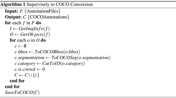
Our algorithm converts annotations from the Supervisely format to the COCO format. For each annotation file, we extract image-level and object-level information. These details are transformed and collected into a new COCO object, which is added to a set of COCO annotations. The process repeats for each object in all annotation files. Finally, the complete set of COCO annotations is saved for future use. The conversion process ensures that all relevant image-level and object-level information is accurately preserved in the resulting COCO annotations.

After the dataset preparation, we trained a model to predict the bounding boxes and segmentation pixels for the objects. We first initiate a baseline model previously trained with Detectron2 called Mask RCNN R 50 FPN model in order to have better tradeoffs between speed and accuracy (Wu et al., 2019) . The model’s training parameters have a batch size of 8, a learning rate of 25 × 10⁻⁵, and a stochastic gradient descent optimizer. We kept the original resolution of the input images and trained the model for 3000 iterations on the available Google Colab¹¹ GPU, taking approximately three and half hours to train.

For better visualization and understanding, Table 2 encapsulates all the hyperparameters tailored for each model of our experiments, where LR stands for Learning Rate and the value LR Finder means that used the learning rate finder technique describe in (Smith, 2017) .

4. Results

In this section we present the achieved results of our initial experiments in the same manner, separating into the two different categories, Semantic and Instance Segmentation. We present a quantitative summary of the performed experiments explaining the metrics. For qualitative analysis we present graphical results emphasizing the problems observed.

4.1. Semantic Segmentation

The evaluation was conducted on a test dataset and the performance of each model was measured in terms of mean Intersection over Union (mIoU), accuracy, and F-score. We selected these metrics as they are commonly used for Semantic Segmentation and they best represent both the successes and errors of models.

Table 3 summarizes the overall performance of the best models we tested. We identified each model with a unique Id for later reference in the paper. Model b, which is the combination of U-net and Resnet18, achieved the highest mIoU of 0.6, an accuracy of 0.8564 and F-score of 0.7234, indicating its overall strong performance and generalization across the entire dataset.

The HRNet model achieved a mIoU of 0.3889, an accuracy of 0.7316, and an F-score of 0.4869 over the test dataset. These results were obtained after training the network for 63,300 epochs.

The U-net and Resnet experiments had different results with different resolutions, as expected. However, we can verify in Table 4 that the model that achieved

Table 2. Hyperparameters for all models developed.

Table 3. Average results of the best models over the test dataset.

Table 4. Quantitative results of the best U-net models for each architecture and resolution.

the best quantitative metrics is the second simplest model is model b, composed of a Resnet18 with 486 × 648 resolution. This model achieved an average IoU of 0.6 across the entire test dataset. In contrast, the Resnet model with 18 residual layers and 972 × 1296 resolution presented only a slight improvement over the model using 243 × 324 resolution.

For better visualization, we present a comparison of quantitative results by model in Table 5. This table shows the results of the best models over the test dataset for each class. Model b outperformed the other models once again, in most of the classes, achieving the highest mIoU and precision for the Tree and Background classes, as well as the highest precision for the Estratocumuliform and Cirriform classes. Model b also achieved the highest recall for the Tree and Background classes, and the highest recall for the Estratiform and Estratocumuliform classes.

Model d, which consisted of an Unet architecture combined with an EfficientNet backbone, achieved a mIoU of 0.4187, an accuracy of 0.8141, and F-score of 0.4871 over the test dataset at the last epoch which was trained on. However, this model also presents problems with segmenting certain classes.

Figure 3 presents the predicted segmentation of each model on the same input image. The Estratiform class is predominant overall with a small area of Cirriform clouds on another layer, behind the main clouds. We can see that no model was able to identify the latter, with only model c inferring classes Cumuliform and Stratiformes, however none are present in the input image. We can also observe that models a, b and d make very similar predictions, however, if we look closely we can see that model a makes a more refined prediction, at the pixel level. Model b and d are more similar to our ground truth mask, hence we

Table 5. Results of the best models over the test dataset, by class.

Figure 3. Predicted cloud segmentation of different models on the same input image, showing the predominance of Estratiform class and the differences in segmentation performance between models.

believe that this is one of the main reasons that model b outperforms the other models.

However, that’s not always the case. We can see in Figure 4 that model a makes wrong predictions, resulting in a much rougher inference, especially over the clouds of class Cumuliform. Models b and c have small patches of this class inside the predicted Estratocumuliform class, which is not correct. This shows the “localization” problem mentioned previously. The model is not able to discern that there are two main cloud objects of the same class. The models are probably being influenced more by texture and shape than other characteristics. We can also see that this problem occurs with small clouds as well, the Estratiform clouds below the main clouds are classified as Estratocumuliform, Estratiform and Cirriform, all in the same small region. Model b is able to classify more parts of the Estratiform clouds correctly, however, only model a is able to detect the faint areas of these clouds at the lower level, even though it classified it incorrectly.

Figure 5 shows two examples of segmentation inference of the best overall model (b). In contrast, the Resnet model with 18 residual layers and 972 × 1296 resolution presented only a slight improvement over the model using 243 × 324 resolution. With this model, it barely segment the most predominant class in the dataset, the Tree class.

The results achieved using the Resnet with 34 residual layers architecture (model c) were not so positive. Figure 6 shows an example of inference using the best models with 486 × 648 (top) and 972 × 1296 (bottom) resolution. All

Figure 4. Example of model’s inference with incorrect predictions for Cumuliform clouds and localization problem.

Figure 5. Example of resulting segmentation inference using the Resnet18 with 486 × 648 resolution model (b).

resulting inferences presented the same problem with poor segmentation, with the model barely able to identify the Tree class.

The EfficientNet model achieved an average mIoU of 0.3622 and we can see an example of a good segmentation on Figure 7 (top). The model performs well when inferring the class with more training samples, Estratocumuliform. Even though the resulting segmentation is not very fine where patches of the sky appear in the middle of the thin clouds atop the image, the model is able to make fine segmentation with the Tree class at the bottom. Some very distant clouds on the horizon were not segmented as well. However, the struggle to segment well the less represented classes is clearly visible (bottom). This result shows that the model is capturing some information about the Estratiform class, but still making incorrect inferences over the same cloud, giving preference to the more predominant class. The same occurs at the top of the image, only this time the model was able to identify only a very small patch of the correct Cirriform class

Figure 6. Example of inference results with 486 × 648 resolution (top) and 972 × 1296 resolution (bottom), using the Resnet with 34 residual layers architecture. The latter corresponds to model c discussed previously.

Figure 7. Example of good and bad resulting segmentation inference with U-net and EfficientNet model.

and wrongly segmented the cloud, similar to the bottom cloud. The model captures information about the Cirriform class and segments the same cloud into two different classes. This is most likely due to the thin texture of these clouds, which in our opinion is an understandable mistake.

4.2. Instance Segmentation

The model was assessed for Average Precision (AP) after training using the COCOEvaluator class in Detectron2 (Lin et al., 2014) . The results can be seen in Table 6, where Type represents the type of result, which can be: bounding boxes results or segmentation pixels. The category represents one of the 5 classes, in which the “Tree” category represents trees and buildings and the remaining 4 classes are cloud types. We empirically used a threshold of 80% for inference.

We can see that the Tree class has the highest score, which is expected since the trees and buildings are virtually static, are present in basically all images, and can be easily distinguishable from clouds. Following that we have the Estratocumuliform class as the cloud class with the highest score, this is likely due to the abundance of images with this type of cloud in the dataset. This class is present in 81.53% of the entire dataset. The classes Estratiform and Cirriform are present in 27.21% and 28.61% of the images in the dataset, respectively. However we can see that, even though we have basically the same amount of images for each class in the dataset, the model can distinguish better Cirriform clouds in both types of results. The Cumuliform class is only present in 9.04% of the images, therefore we believe that the results are a reflection of that as well. Overall results are shown in Figure 8.

We also performed a qualitative evaluation in which we looked for the “localization” problem. We can see the result from examples in Figure 9. This problem is less common with this type of model, however, it’s still present but with different characteristics. On the right side of the image, we can observe a detection of multiple Estratocumuliform clouds where in fact there’s only one predominant

Table 6. Detectron2 results separated by bounding box and segmentation pixels. Results are given by Average Precision (AP) per image category.

Figure 8. Resulting Detectron2 segmentation examples.

Figure 9. Example of localization problem where one big cloud is classified as two or more clouds of the same type.

large cloud present with a few scattered on top. On the left side, we can see one Cirriform cloud being classified as two objects. We also identified a problem with the detected region, where sometimes the model tends to crop out some parts of the object. We can see some examples of this situation in Figure 10. This is most likely due to the imposed threshold for plotting the bounding boxes. During inference, the threshold is utilized to filter out low-scored bounding boxes predicted by the model’s Fast R-CNN component. Predictions with a confidence score lower than the threshold are discarded, therefore we can have resulting inference with no cloud classification whatsoever.

5. Discussion

Comparing the results of our study with those in the existing literature presents several challenges, primarily due to the unique nature of our dataset and the particularities of cloud classification tasks.

Firstly, the specific conditions that are represented in the dataset have a significant impact on how well cloud classification models perform. The results can be significantly influenced by variables like the frequency of various cloud types, atmospheric conditions, and even the time of year. For instance, a dataset with a high percentage of images showing cirrus clouds that are challenging to categorize or highly turbid weather could result in poorer performance metrics. On the other hand, a dataset with mostly clear skies and recognizable cloud formations might produce better results. Without using the same dataset for evaluation, this variability makes direct comparisons between studies challenging.

Our study differs from most other studies in the field because we chose to use horizon-oriented images. Many studies employ images of the entire sky or of specific areas of the sky. Our method falls somewhere in the middle of these two, offering more context than patch images while falling short of an all-encompassing 360-degree view like ASIs. Comparisons with other studies are made more difficult by the unique perspective’s own set of advantages and difficulties. Additionally, there can be significant differences in the methodologies and performance metrics applied across studies, which further complicates any comparison.

Figure 10. Example of threshold problem where clouds are not classified due to the confidence being lower than the imposed threshold.

We can see in Table 7 that (Fabel et al., 2022) achieved competitive performance in cloud layer classification using both IP-SR* and DC** methods, with average accuracies of 0.8575 and 0.8522, respectively. These results indicate the effectiveness of their approaches in distinguishing cloud layers based on cloud height. In contrast, Ye et al. (2019) utilized a fine-grained algorithm and achieved an average accuracy of 0.7128 for classifying eight different cloud types in a dataset of 500 test images. In our study, our best model employed a U-net architecture in conjunction with ResNet18 (model b) and classified four distinct cloud types. Our proposed methodology achieved a comparable average accuracy of 0.8564 and demonstrated promising performance in terms of average precision, recall, and intersection over union.

The primary reason behind choosing these references for comparison is that they both presented semantic segmentation results, which went beyond binary classification, and showcased good performance. However, it is essential to highlight certain distinctions in their methodologies. In the case of (Fabel et al., 2022) , the authors focused on cloud layer classes, utilizing cloud height as the basis for their classification. While their approach provided valuable insights into the vertical distribution of clouds, it did not differentiate between different cloud types within the same layer. This limitation is significant as it hampers a more fine-grained analysis of cloud properties and their associated effects. On the other hand, Ye et al. (2019) employed a more comprehensive classification scheme, incorporating four additional classes compared to our study. This expanded categorization allowed for a more detailed representation of cloud types and their respective characteristics. By encompassing a broader range of cloud classes, Ye et al. (2019) captured a more nuanced understanding of cloud patterns and behaviors, which may have implications for various applications. Since both (Fabel et al., 2022) and (Ye et al., 2019) compare their results to other studies in their respective papers, it establishes a precedent for further comparative analysis. By following this approach, we can extend the comparison and evaluate our results in relation to additional relevant studies in the field.

By juxtaposing our results against these two works, we aimed to provide a thorough evaluation of our methodology’s effectiveness and identify potential areas for improvement. Our comparison underscores the importance of considering

Table 7. Comparative analysis of results between our study and the literature in terms of class type, methodology, number of images used for testing, and performance metrics including Average Accuracy (AA), Average Precision (AP), Average Recall (AR), and Average Intersection over Union (AIoU).

both cloud layer distinctions and a diverse set of cloud classes in semantic segmentation tasks, enabling a more comprehensive analysis of cloud-related phenomena.

Compared to the experiments performed during the exploratory phase of our research, we can see an improvement in overall metrics and the quality of the segmentation. It is clear to us that our problem of cloud segmentation does not need a complex architecture like the Resnet with 34 residual layers. On the contrary, we believe that it is best to keep the architecture simple. A lower resolution might also improve the performance compared to models using higher a resolution due to the resulting segmentation being too fine-grained. This can result in a performance drop in the final results with such high resolution test images and the fact that the ground-truth annotations are not that precise. It is worth mentioning that the Tree class is creates a favorable bias for the overall results of all models. Quantitatively speaking, the best overall model is model b, which is a U-net with Resnet18 using 486 × 648 resolution. It performed an average IoU of 0.6. We can argue that model a, the HRNet model, also performs well, since it gives a finer segmentation inference (with higher resolution), even though it performs poorly with an average IoU of 0.3889. Even though the Detectron2 model had good results for the tree class, it performed poorly for the remaining classes and presented some issues regarding the fixed threshold and localization problem, which was the main reason we opt to experiment with this model.

The achieved results have raised questions about why a simpler model outperforms a more complex one, leading to the need for future investigations. Six potential causes were identified for further exploration: 1) Overfitting, as complex models with more parameters are prone to overfitting, while simpler models can generalize better; 2) Appropriate complexity, where the task of cloud segmentation may not be as complex for a machine learning model as initially thought; 3) Data availability, as complex models require more data to learn effectively, while simpler models may perform better with limited data; 4) Hyperparameter tuning, since complex models have more hyperparameters that need optimal tuning for optimal performance; 5) Regularization techniques like dropout, weight decay, or early stopping, which can prevent overfitting in complex models; and 6) Data quality, where a simpler model may be more robust against noisy data. These factors will be addressed in future works to gain further insights.

An important disclaimer is that no detailed analysis was performed to validate if the results were actually representing the clouds better than the ground truth. Despite this, a few examples were detected, and the decision to include different models as part of the experiment was made, with the intent to reduce the problem as much as possible.

6. Conclusion

The initial experiments showed that it is possible and feasible to classify clouds using current techniques of machine learning. Flat cameras pointing to the horizon allowed us to observe vertical distribution for classification, avoided image distortion of fish-eye lenses, and simplified image processing. We could see that the results were positive overall, even for initial results. This was a good proof of concept in the sense of giving us a better understanding of what techniques work best. Both models had satisfactory results for initial experiments, but it is evident that the data imbalance is affecting the performance. The HRNet model looks more promising as it works with different resolutions, thus leading to a more refined segmentation, at the pixel level. However, it seems that such an intricate model is not necessary in order to detect the most predominant clouds in the sky. We were able to achieve the best results with a simpler model, using a much lower resolution. This can be useful in the future since our main objective is to use such models to predict cloud motion and forecast the impact it will have on solar power generation. We mapped out the data augmentation transformations for our next experiments and are currently working on balancing the dataset. We will also consider removing the Tree class in order to obtain more realistic results. For future studies, a better overall cloud classification model will be researched and developed based on the results presented here.

7. Future Work

In this work, we focused on well-established semantic segmentation approaches. Since 2019, however, Vision Transformers (ViTs), a paradigm originally from the Natural Language Processing (NLP) field, have been applied with success to image processing and have achieved better results than “traditional” CNN models like ours on reference image datasets (Dosovitskiy et al., 2021) . Transformers have been used for NLP in the last few years and have gotten very promising results in this field. One important feature in the transformer models is the attention mechanism that gives more value to some data than others. This process can lead to better results as the model might take the most important data more into account, instead of working equally with all of it (Wolf et al., 2020) . The observed improvement aligns with the architectural distinctions between Convolutional Neural Networks (CNNs) and Vision Transformers (ViTs). While CNNs leverage convolutional layers to process spatial information in a local and hierarchical manner, ViTs employ self-attention mechanisms to process spatial relationships globally across the image. Specifically, CNNs operate on local receptive fields and aggregate spatial hierarchies layer-by-layer, whereas ViTs have the capacity to attend to any part of the image regardless of the spatial position, thereby enabling a global understanding of spatial dependencies. Consequently, ViTs may exhibit enhanced performance in certain image processing tasks that benefit from such global spatial processing. However, this type of model needs more data and training time to learn those relationships. For this reason, the ViT was not chosen for our initial set of experiments. In future work, we plan to compare results to be obtained with ViTs against the models presented in this work.

The present work used image validation based on a senior synoptic observer who trained the marking image team. But in the future, we are considering using additional equipment like LIDAR, stereo cameras, satellite images or sounding balloons that could help validate the developed methodology.

Dataset Additional Improvements

At the time of the experiments, our dataset was composed of 996 fully hand-annotated images, ranging from March to October of 2021. We are currently finishing annotating more images and intend to publish the new images soon. We understand that it is important to have at least one year of images to capture the different seasons. The dataset is unbalanced due to the lack of typical clouds that form more often during the southern hemisphere summer. These newly captured images will be used in future experiments, and we hope to mitigate this problem. Data augmentation can also help, but only a few transformations can be performed on the dataset. For example, we cannot flip the image vertically, only horizontally. We mapped out: horizontal flip; brightness; contrast; Hue, Saturation, and Value (HSL); gamma; and the application of contrast-limited adaptive histogram equalization, as possible transformations. This dataset will be regularly improved, and we aim to increase its representativeness. New versions will be made available as soon as they have undergone review.

Acknowledgements

The authors would like to thank Dr. Maurici Amantino Monteiro climatologist at Aqueris Engenharia e Soluções Ambientais. His years of experience in synoptic observations helped us in the initial phase to understand the nature of clouds and their association with corresponding classes.

We also thank our Data Analysts: Marco Polli, Thiago Chaves and Nicolas Moreira Branco for the great work with producing the Clouds-1000 dataset used in this work.

NOTES

¹https://public.wmo.int/en

²https://cloudatlas.wmo.int/en/cloud-classification-summary.html

³https://www.cityscapes-dataset.com/

⁴https://en.climate-data.org/south-america/brazil/santa-catarina/florianopolis-1235/

⁵https://education.nationalgeographic.org/resource/koppen-climate-classification-system/

⁶https://supervise.ly/

⁷https://github.com/PaddlePaddle/PaddleSeg

⁸https://www.fast.ai/

⁹https://github.com/facebookresearch/detectron2

¹⁰https://cocodataset.org/

¹¹https://colab.research.google.com/

Conflicts of Interest

The authors declare no conflicts of interest regarding the publication of this paper.

References

[1]	Alvares, C. A., Stape, J. L., Sentelhas, P. C., de Moraes Gonçalves, J. L., & Sparovek, G. (2013). Köppen’s Climate Classification Map for Brazil. Meteorologische Zeitschrift, 22, 711-728. https://doi.org/10.1127/0941-2948/2013/0507
[2]	Anagnostos, D., Schmidt, T., Cavadias, S., Soudris, D., Poortmans, J., & Catthoor, F. (2019). A Method for Detailed, Short-Term Energy Yield Forecasting of Photovoltaic Installations. Renewable Energy, 130, 122-129. http://www.sciencedirect.com/science/article/pii/S0960148118307109
[3]	Barrett, E., & Grant, C. K. (1976). The Identification of Cloud Types in Landsat MSS Images. Tech. Rep.
[4]	do Nascimento, L. R., Braga, M., Campos, R. A., Naspolini, H. F., & Rüther, R. (2020). Performance Assessment of Solar Photovoltaic Technologies under Different Climatic Conditions in Brazil. Renewable Energy, 146, 1070-1082. https://www.sciencedirect.com/science/article/pii/S0960148119310006
[5]	do Nascimento, L. R., de Souza Viana, T., Campos, R. A., & Rüther, R. (2019). Extreme Solar Overirradiance Events: Occurrence and Impacts on Utility-Scale Photovoltaic Power Plants in Brazil. Solar Energy, 186, 370-381. https://www.sciencedirect.com/science/article/pii/S0038092X19304530
[6]	Dosovitskiy, A., Beyer, L., Kolesnikov, A., Weissenborn, D., Zhai, X., Unterthiner, T. et al. (2021). An Image Is Worth 16x16 Words: Transformers for Image Recognition at Scale. http://arxiv.org/abs/2010.11929
[7]	Dubreuil, V., Fante, K., Planchon, O., & Santa’Anna Neto, J. (2018). The Types of Annual Climates in Brazil: An Application of the Classification of Köppen from 1961 to 2015. EchoGéo. https://doi.org/10.4000/echogeo.15017
[8]	Fabel, Y., Nouri, B., Wilbert, S., Blum, N., Triebel, R., Hasenbalg, M. et al. (2022). Applying Self-Supervised Learning for Semantic Cloud Segmentation of All-Sky Images. Atmospheric Measurement Techniques, 15, 797-809. https://amt.copernicus.org/articles/15/797/2022/
[9]	Haeffelin, M., Barthès, L., Bock, O., Boitel, C., Bony, S., Bouniol, D., et al. (2005). SIRTA, A Ground-Based Atmospheric Observatory for Cloud and Aerosol Research. Annales Geophysicae, 23, 253-275. https://angeo.copernicus.org/articles/23/253/2005/angeo-23-253-2005.html
[10]	Hu, Y., & Stamnes, K. (2000). Climate Sensitivity to Cloud Optical Properties. Tellus B, 52, 81-93. https://doi.org/10.3402/tellusb.v52i1.16084
[11]	Juncklaus Martins, B., Cerentini, A., Neto, S. M., & von Wangenheim, A. (2021). Systematic Literature Review on Forecasting/Nowcasting Based upon Ground-Based Cloud Imaging. https://www.researchgate.net/publication/349536859_Systematic_Literature_Review_on_ForecastingNowcasting_based_upon_Ground-Based_Cloud_Imaging
[12]	Juncklaus Martins, B., Cerentini, A., Neto, S. M., & von Wangenheim, A. (2022a). Systematic Review of Nowcasting Approaches for Solar Energy Production Based upon Ground-Based Cloud Imaging. Solar Energy Advances, 2, Article 100019. https://doi.org/10.1016/j.seja.2022.100019
[13]	Juncklaus Martins, B., Polli, M., Cerentini, A., Mantelli, S., Chaves, T., Moreira Branco, N. et al. (2022b). Clouds-1000. Mendeley Data. https://data.mendeley.com/datasets/4pw8vfsnpx/1
[14]	Kumari, P., & Toshniwal, D. (2021). Deep Learning Models for Solar Irradiance Forecasting: A Comprehensive Review. Journal of Cleaner Production, 318, Article 128566. https://www.sciencedirect.com/science/article/pii/S0959652621027736
[15]	Li, P., Dong, L., Xiao, H., & Xu, M. (2015). A Cloud Image Detection Method Based on SVM Vector Machine. Neurocomputing, 169, 34-42. http://www.sciencedirect.com/science/article/pii/S0925231215006864
[16]	Lin, T., Maire, M., Belongie, S., Hays, J., Perona, P., Ramanan, D. et al. (2014). Microsoft Coco: Common Objects in Context. In D. Fleet, T. Pajdla, B. Schiele, & T. Tuytelaars (Eds.), European conference on Computer Vision (pp. 740-755). Springer. https://doi.org/10.1007/978-3-319-10602-1_48
[17]	Long, C. N., Sabburg, J. M., Calbo, J., & Page, J. D. (2006). Retrieving Cloud Characteristics from Ground-Based Daytime Color All-Sky Images. Journal of Atmospheric and Oceanic Technology, 23, 633-652. https://doi.org/10.1175/JTECH1875.1
[18]	Mantelli, S. L., von Wangenheim, A., Pereira, E. B., & Sobieranki, A. C. (2020). Hierarchical Color Similarity Metrics for Step-Wise Application on Sky Monitoring Surface Cameras. Earth and Space Science Open Archive. https://doi.org/10.1002/essoar.10503135.1
[19]	Mantelli, S. L., von Wangenhein, A., Pereira, E. B., & Comunello, E. (2010). The Use of Euclidean Geometric Distance on RGB Color Space for Classification of Sky and Cloud Patterns. Journal of Atmospheric and Oceanic Technology, 27, 1504-1517. https://doi.org/10.1175/2010JTECHA1353.1
[20]	Martins, G. L., Mantelli, S. L., & Rüther, R. (2022). Evaluating the Performance of Radiometers for Solar Overirradiance Events. Solar Energy, 231, 47-56. https://www.sciencedirect.com/science/article/pii/S0038092X21010100
[21]	Mejia, F. A., Kurtz, B., Murray, K., Hinkelman, L. M., Sengupta, M., Xie, Y., & Kleissl, J. (2016). Coupling Sky Images with Radiative Transfer Models: A New Method to Estimate Cloud Optical Depth. Atmospheric Measurement Techniques, 9, 4151-4165. https://www.atmos-meas-tech.net/9/4151/2016/
[22]	Mellit, A., & Kalogirou, S. A. (2008). Artificial Intelligence Techniques for Photovoltaic Applications: A Review. Progress in Energy and Combustion Science, 34, 574-632. http://www.sciencedirect.com/science/article/pii/S0360128508000026
[23]	Monteiro, M. A. (2001). Caracterizacao climatica do estado de santa catarina: Uma abordagem dos principais sistemas atmosfericos que atuam durante o ano. Geosul, 16, 69-78.
[24]	Paletta, Q., & Lasenby, J. (2020). Convolutional Neural Networks Applied to Sky Images for Short-Term Solar Irradiance Forecasting. arXiv:2005.11246 https://arxiv.org/abs/2005.11246
[25]	Pelland, S., Remund, J., Kleissl, J., Oozeki, T., & De Brabandere, K. (2013). Photovoltaic and Solar Forecasting: State of the Art. https://iea-pvps.org/wp-content/uploads/2013/10/Photovoltaic_and_Solar_Forecasting_State_of_the_Art_REPORT_PVPS__T14_01_2013.pdf
[26]	Piccardi, M. (2004). Background Subtraction Techniques: A Review. In 2004 IEEE International Conference on Systems, Man and Cybernetics (Vol. 4, pp. 3099-3104). IEEE. https://doi.org/10.1109/ICSMC.2004.1400815
[27]	Ronneberger, O., Fischer, P., & Brox, T. (2015). U-Net: Convolutional Networks for Biomedical Image Segmentation. In N. Navab, J. Hornegger, W. Wells, & A. Frangi (Eds.), Medical Image Computing and Computer-Assisted Intervention. Lecture Notes in Computer Science (Vol. 9351, pp. 234-241). Springer. https://doi.org/10.1007/978-3-319-24574-4_28
[28]	Smith, L. N. (2017). Cyclical Learning Rates for Training Neural Networks. In 2017 IEEE Winter Conference on Applications of Computer Vision (WACV) (pp. 464-472). IEEE. https://doi.org/10.1109/WACV.2017.58
[29]	Souza-Echer, M. P., Pereira, E. B., Bins, L., & Andrade, M. A. R. (2006). A Simple Method for the Assessment of the Cloud Cover State in High-Latitude Regions by a Ground-Based Digital Camera. Journal of Atmospheric and Oceanic Technology, 23, 437-447. https://doi.org/10.1175/JTECH1833.1
[30]	Tan, M., & Le, Q. V. (2019). EfficientNet: Rethinking Model Scaling for Convolutional Neural Networks. https://arxiv.org/abs/1905.11946
[31]	Tarrojam, B., Mueller, F., Eichman, J. D., & Samuelsen, S. (2012). Metrics for Evaluating the Impacts of Intermittent Renewable Generation on Utility Load-Balancing. Energy, 42, 546-562. http://www.sciencedirect.com/science/article/pii/S0360544212001351
[32]	Voyant, C., Notton, G., Kalogirou, S., Nivet, M., Paoli, C., Motte, F., & Fouilloy, A. (2017). Machine Learning Methods for Solar Radiation Forecasting: A Review. Renewable Energy, 105, 569-582. https://www.sciencedirect.com/science/article/pii/S0960148116311648
[33]	Wolf, T., Debut, L., Sanh, V., Chaumond, J., Delangue, C., Moi, A. et al. (2020). Transformers: State-of-the-Art Natural Language Processing. In Proceedings of the 2020 Conference on Empirical Methods in Natural Language Processing: System Demonstrations (pp. 38-45). Association for Computational Linguistics. https://aclanthology.org/2020.emnlp-demos.6
[34]	Wu, Y., Kirillov, A., Massa, F., Lo, W.-Y., & Girshick, R. (2019). Detectron2. https://github.com/facebookresearch/detectron2
[35]	Ye, L., Cao, Z., Xiao, Y., & Yang, Z. (2019). Supervised Fine-Grained Cloud Detection and Recognition in Whole-Sky Images. IEEE Transactions on Geoscience and Remote Sensing, 57, 7972-7985. https://doi.org/10.1109/TGRS.2019.2917612
[36]	Yuan, Y., Chen, X., & Wang, J. (2020). Object-Contextual Representations for Semantic Segmentation. In A. Vedaldi, H. Bischof, T. Brox, & J. M. Frahm (Eds.), Computer Vision. Lecture Notes in Computer Science (Vol. 12351, pp. 173-190). Springer. https://doi.org/10.1007/978-3-030-58539-6_11