An Agent-Based Approach to the Newsvendor Problem with Price-Dependent Demand

Patrick R. McMullen

School of Business, Wake Forest University, Winston-Salem, USA.

DOI: 10.4236/ajor.2020.104006                

Abstract

This research presents an agent-based approach to finding near-optimal solutions to the newsvendor problem with price-dependent demand. The classical newsvendor problem is pursued where the decision of order quantity needs to be made in order to maximize expected profit. Here, the additional caveat of price-sensitive demand is included. This means that price (P) and order quantity (Q) are decision variables under the control of the newsvendor, with the intent of maximizing the expected value of the associated profit. The solution approach exploits an agent-based strategy, where an artificial agent traverses a grid-coordinate system of Price and Quantity values, where each unique Price and Quantity combination results in an expected profit. The agent-based approach consistently results in optimal solutions to a problem from the literature.

Keywords

Optimization, Heuristic, Search

1. Introduction

The classical newsvendor (formerly known as “newsboy”) problem involves individual selling items on a periodic basis (such as daily newspapers). The individual needs to determine how many items to purchase to re-sell in the face of uncertain demand to maximize the expected profit [1]. If the individual purchases too many items, supply exceeds demand, and the excess supply must be discarded or sold at a loss. If the individual purchase too few items, demand exceeds supply, and opportunity loss occurs. As such, deciding the “best” purchase quantity is of great importance.

Another variable to consider is the price. A fundamental law of economics tells us that for commodity items, demand decreases as price increases. Conversely, demand increases as price decreases [2] [3] [4]. As such, it stands to reason that for the newsvendor problem, choosing an appropriate price in addition to choosing an appropriate quantity are decision variables that must be taken quite seriously. In the face of all of this, we cannot forget that while choosing the appropriate values of quantity and price, we must also realize that demand is a stochastic quantity that we cannot predict with certainty [5] [6] [7].

Because of these decision variables in the face of uncertainty, we need to pursue a solution approach that considers these entities simultaneously. This is the theme of this research effort. The approach presented here exploits an agent-based approach—something in the spirit of Ant Colony Optimization, or similar [8] [9]. Ant Colony Optimization (ACO) can be thought of as a branch of Swarm Intelligence. Swarm Intelligence exploits the behavior of social insects like ants, bees termites, etc. As individuals, these insects are blind, deaf and in short, have limited functional ability. However, they have a profound ability to communicate by their movements. This communicative ability alerts other members of the swarm as to the most efficient ways to complete tasks, such as finding food, avoiding predators, etc. As a swarm, these insects exhibit collective intelligence, and their behavior is used by researchers and practitioners to address complex problems [10] [11] [12]. Specifically, an artificial agent will traverse a space, where each point in space is a specific combination of price and quantity. Each point in space also has an expected value of profit. The intent is to find the unique combination of price and quantity that maximizes the expected profit. It is the author’s opinion that the unique contribution of this paper is the use of swarm intelligence to address an important problem in optimization and inventory management. Additionally, the use of a heat map is helpful in visualizing a complex problem.

The subsequent sections of this paper explain the methodology used in terms of the profit function dependent on price and quantity, describe the development of the space representing price, quantity and expected profit, and describe the agent-based simulation model used to finding the value of price and quantity that maximizes the expected profit. Conclusions are also offered and opportunities for subsequent research are also discussed.

2. Methodology

The methodology used for this effort is essentially comprised of three parts: the first part details the newsvendor model with price-sensitive demand; the second part details the construction of the search space for the artificial agent; and the third part details the simulation model used to guide the artificial agent’s search for optimality.

2.1. Newsvendor Model with Price-Sensitive Demand

The newsvendor problem, in the context of this research strives to maximize profit associated with the purchase and subsequent re-selling of some item. With that in mind, the following definitions are provided in Table 1.

Table 1. Newsvendor variables.

As stated previously, demand is stochastic and price-sensitive. As such, the following relationship more specifically describes demand:

$D=a-bP+\epsilon$ , (1)

where

$\epsilon ~N\left({\mu }_D,{\sigma }_D\right)$ (2)

Combining revenue and cost functions in terms of the above, the following profit function results:

$\pi =\left(P-V+S\right)\ast \min \left(Q,D\right)-SD-\left(C-V\right)\ast Q$ (3)

Ideally, taking the derivative of profit with respect to P and Q and setting these equal to zero, then solving for P and Q is preferred, but the discontinuous nature of the equation, and the fact that D is stochastic, makes this process unrealistic, resulting in conditional approaches [6]. As such, a more “brute-force” is pursued.

2.2. Search Space for Artificial Agent

In order to have an artificial agent search for a combination of price and quantity, a search space must be constructed. In order to do this, the following definitions are provided in Table 2.

The number of subintervals, n, is the same for both price and quantity so that the search grid is square. The pseudocode to determine the grid values is as follows:

for i = 0 to n {

P = P_min + i × ((P_max − P_min)/n)

for j = 0 to n {

Q = Q_min + j × ((P_max − P_min)/n)

for k = 1 to m {

calculate π(P, Q)}

calculate $\bar{\pi }$ , s

}}

calculate ρ

Table 2. Search grid construction definitions.

For each unique combination of P and Q, the value of π is computed m times. This is done to account for the stochastic nature of Demand (D). As such, profit is simulated for each combination of P and Q, resulting in subsequent values of $\bar{\pi }$ .

The pseudocode above provides (n + 1)² grid points. Each grid point has values of P, Q, $\bar{\pi }$ , and s. In addition, the percentile rank (ρ) for profit is calculated for each of the (n + 1)² grid points.

The end-result is a grid that takes on the following general structure:

2.3. Artificial Agent’s Search for Optimality

At this point there is an (n + 1) by (n + 1) search grid for the artificial agent to traverse. To repeat, each grid point has a value of P, Q, $\bar{\pi }$ , s and ρ. The intent is to create an artificial agent to find the grid point where $\bar{\pi }$ is maximized. The definitions in Table 3 detail the terminology used for the artificial agent search— some the variables at the bottom are “re-defined” for the purpose of classifying them as grid-oriented terms.

The following subsections describe the search associated with the artificial agent.

2.3.1. Initialization

Prior to the commencement of the search, several terms are initialized. Values of P, Q, $\bar{\pi }$ , s and ρ, as described in the previous section are used as values for their respective grid points. The visitation index (𝓋) for each grid point is initialized to 1. The agent index (𝒶) is initialized to 1 [9].

2.3.2. Create Agent

An artificial agent is created and located at a random position on the Price-Quantity (P, Q) grid. The time index (t) is initialized to zero.

Table 3. Artificial agent definitions.

2.3.3. Move Agent

The agent moves to a neighboring grid point. Figure 1 details agents and neighboring grid points.

In this figure, there are several artificial agents shown, denoted by letters, and in black cells. Each agent has neighboring grid points—points that are adjacent to the agent, and these cells are grey. There are agents in the corners of the grid (I, K, A and D), and each of these agents have three neighbors. There are agents on the edge of the grid (J, E, H and B), and each of these agents have five neighbors. There are agents in the middle of the grid (L, C, F, M, G), and these agents each have eight neighbors. Regardless of where the agent is located, the agents that are neighbors of the current agent are in the set S.

The current agent will move to a neighboring grid point. Monte-Carlo simulation is used to select the neighbor. Neighbor i of the current agent has the following probability of being selected:

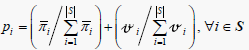(4)

This probability has two components. The first component is the relative desirability of the expected profit of neighbor i. The second component relates to the relative desirability of neighbor i. This of relative desirability of neighbor i as a surrogate measure of pheromone—a tool used to encourage or discourage possible grid points.

The agent moves to the chosen neighboring grid point. The values of P, Q, $\bar{\pi }$ , s and ρ for the new grid point are already known. The profit associated with the new grid point is π_C. If this value of π_C is the best profit thus far, the value of π_B is

Figure 1. Agents and neighboring grid points.

replaced with the value of π_C. If the percentile rank value of the new grid point (ρ) exceeds a threshold value (τ), the following adjustment occurs:

𝓋 = (1 + α) (5)

Otherwise, this adjustment occurs:

𝓋 = (1 − α) (6)

This adjustment of the visitation (or pheromone) index is done to enhance desirable grid points, and to reduce less desirable grid points.

If the value of 𝒶 is equal to A, the simulation is over, and all relevant outputs are reported. Otherwise, 𝒶 is incremented by 1 (𝒶 = 𝒶 + 1). If the value of t is equal to T, the current agent is terminated, and control is returned to subsection 2.3.2. Otherwise, t is incremented by 1 (t = t + 1) and control is returned to subsection 2.3.3.

If the value of t is equal to the value of T, then the agent terminates, and control is returned to subsection 2.3.2.

2.3.4. End of Simulation

Upon the end of the simulation, several values are noted: the overall best profit found (π_B), the Price and Quantity values associated with this profit (P and Q), and the percentage of agents that exceed the threshold value (τ) during the simulation.

3. Experimentation

The methodology presented above was carried-out via experimentation. A problem from the literature was used as an example [13]. The profit model terms took on the values shown here in Table 4:

Table 4. Artificial agent search values.

The values above were substituted into Equation (3), with P and Q as variables. There are 301 values for both P and Q. Each P, Q combination was used and profit was simulated m = 250 times. This was done to get reliable estimates for both $\bar{\pi }$ and s for each P, Q combination. This results in a grid of (301 × 301 = 90,601) grid points. After the grid points were generated via simulation, the percentile values in terms of $\bar{\pi }$ were then determined and recorded as ρ. The above data set (grid values) was generated via the Java Programming Language.

In terms of using artificial agents to find the values of P and Q that maximize $\bar{\pi }$ , an environment was constructed using NetLogo, a software package that specializes in Agent -Based modeling [14]. Experimentation was used to arrive at the model parameter values that provides consistently desirable solutions. These parameter values are detailed in Table 5.

Figure 2 shows the P, Q search grid. The horizontal axis shows the values of P, while the vertical axis shows the values of Q.

The coloration of the grid emulates a heat map, intended to show relative values of expected profit ( $\bar{\pi }$ ). In this context, the heat map represents three-dimensional data [15]. The horizontal axis is Price, the vertical axis is Quantity, while the third axis, the one perpendicular to the page is expected profit ( $\bar{\pi }$ ). The darker the value, the higher the expected profit. This heat map is colored in such a way that the ant seeks to find the darkest part of the heat map. Also shown is an artificial agent—in this case an ant is chosen as the artificial agent, due to the ant’s attraction to pheromone. The agent appears to be headed to a “good” solution in terms of maximum profit—that is, the ant is moving toward the darkest red area.

4. Experimental Results

The search parameters above show that each agent had a lifetime of (2000) time units, and each simulation used (50) agents. Experimentation showed the most favorable threshold value (τ) was 0.72, with the most favorable amplifier value (α) to be 0.009. The NetLogo simulation was performed 200 times at these settings,

Table 5. Values of experimental variables.

Figure 2. Search grid for artificial agent.

and the average profit was found to be $359.17, with the optimal profit being $359.29. A formal hypothesis test was performed to see if this average profit found was statistically different from the optimal of $359.29. The test is as follows:

${\text{H}}_0:\mu =359.29;{\text{H}}_{\text{A}}:\mu <359.29$ (7)

The above provided a test statistic of t = −0.29, with an associated p-value of 0.3842. As such, we cannot reject the H₀, which enables us to claim our results are no different from optimal.

Another performance-related metric that was studied was the percentage of agents that met the threshold (τ) during the simulation. During the simulation, there is no guarantee an agent will find the optimal solution. In fact, there is no guarantee that an agent will even find a good solution. This is because the agent is randomly assigned a starting point, and the agent’s movements are always random to some degree. This fact is the very reason that multiple agents are used in a simulation. For this effort, it was discovered that 92.46% of the ants simulated met the threshold of τ, which was the 72^nd percentile. The standard deviation was 3.53% of the agents. It turns out that finding the optimal solution was easier than finding a high-value of agents that met the threshold value of τ. The percentage of agents meeting the threshold of τ is considered a measure of robustness for the approach. The values of τ and α essentially control the amount of pheromone associated with each of the grid points. The combination of τ = 0.72 and α = 0.009 was the result of rigorous experimentation.

5. Concluding Comments

Methodology has been presented to address the newsvendor problem with Price-Sensitive and stochastic demand. An agent-based approach is employed to provide a novel search approach to the problem with essentially optimal results.

One of the unique things associated with the test problem is that we (as observers) already know the optimal solution before we pursue the optimal solution via the artificial agent search. Because the artificial agent is “blind,” we find this approach reasonable. The blindness of the artificial agent exists because the agent does not know where the optimal solution is—only the observer knows this. The agent only knows about properties of neighboring grid points (values of P and Q), and behaves accordingly. The challenge of the agent-based approach is to instruct the agent to find the optimal solution via the most efficient-possible means. For larger, perhaps more “real-world” types of problems the observer is much less likely to know the optimal solution. This is a common trait for problems of the “hill-climbing variety.”

This effort presents many opportunities for subsequent research. The normal distribution was used here to model the stochastic nature of demand (D). There are, of course, other distributions that could be used to model demand (exponential, etc.). There are other types of agent-based approaches that could be used to find optimal and/or desirable solutions. Specifically, other mechanisms to emulate pheromone could be explored. Additionally, other, particularly larger, problems could be addressed. Also, our profit function was expressed in expected profit ( $\bar{\pi }$ )—this means that there is a degree of uncertainty associated with expected profit. A different objective function, considering the degree of variation associated with the expected value, could be considered an opportunity for subsequent research.

In summary, the conclusions can be condensed as follows:

· An agent-based approach is used to address the Price-Sensitive Newsvendor Problem with essentially optimal results and in a computationally-efficient manner.

· There are opportunities for subsequent research involving:

o Various probability distributions could be explored.

o Different pheromone approaches could be studied.

o Larger, more complex problems could be addressed.

o Other objective functions could be pursued.

Conflicts of Interest

The authors declare no conflicts of interest.

References

[1]	Edgeworth, F.Y. (1888) The Mathematical Theory of Banking. Journal of the Royal Statistical Society, 51, 113-127.
[2]	Schulte, B. and Sachs, A. (2020) The Price-Setting Newsvendor with Poisson Demand. European Journal of Operational Research, 283, 125-137. https://doi.org/10.1016/j.ejor.2019.10.039
[3]	Kocabiyikoglu, A. and Popescu, I. (2011) An Elasticity Approach to the Newsvendor with Price-Sensitive Demand. Operations Research, 59, 301-312. https://doi.org/10.1287/opre.1100.0890
[4]	Kocabiyikoglu, A., Gogus, C.I. and Gonul, M.S. (2016) Decision Making and the Price Setting Newsvendor: Experimental Evidence. Decision Sciences, 47, 157-186. https://doi.org/10.1111/deci.12158
[5]	Petruzzi, N.C. and Dada, M. (1999) Pricing and the Newsvendor Problem: A Review with Extensions. Operations Research, 47, 183-194. https://doi.org/10.1287/opre.47.2.183
[6]	Qin, Y., Wang, R., Vakharia, A., Chen, Y. and Seref, M.H. (2011) The Newsvendor Problem: Review and Directions for Further Research. European Journal of Operational Research, 213, 361-374. https://doi.org/10.1016/j.ejor.2010.11.024
[7]	Gallego, G. and van Ryzin, G. (1994) Optimal Dynamic Pricing of Inventories with Stochastic Demand over Finite Horizons. Management Science, 40, 999-1020. https://doi.org/10.1287/mnsc.40.8.999
[8]	Tarasewich, P. and McMullen, P.R. (2002) Swarm Intelligence: Power in Numbers. Communications of the ACM, 45, 62-67. https://doi.org/10.1145/545151.545152
[9]	Bonabeau, E., Dorigo, M. and Theraulz, G. (1999) Swarm Intelligence: From Natural to Artificial Systems. International Journal of Computer Applications in Technology, 12, 320-328.
[10]	Bonabeau, E., Dorigo, M. and Theraulz, G. (1999) Swarm Intelligence: From Natural to Artificial Systems. Oxford University Press, Oxford.
[11]	Deneubourg, J.-L., Aron, S., Goss, S. and Pasteels, J.-M. (1990) The Self-Organizing Exploratory Pattern of the Argentine Ant. Journal of Insect Behavior, 3, 159-168. https://doi.org/10.1007/BF01417909
[12]	Di Caro, G. and Dorigo, M. (1998) AntNet: Distributed Stigmergetic Control for Communications Networks. Journal of Artificial Intelligence Research, 9, 317-365. https://doi.org/10.1613/jair.530
[13]	Lau, A. and Lau, H. (1988) The Newsboy Problem with Price-Dependent Demand Distribution. IIE Transactions, 20, 168-175. https://doi.org/10.1080/07408178808966166
[14]	Wilensky, U. and Rand, W. (2015) An Introduction to Agent-Based Modeling. The MIT Press, Boston.
[15]	Perrot, A., Bourqui, R., Hanusse, N., Lalanne, F. and Auber, D. (2015) Large Interactive Visualization of Density Functions on Big Data Infrastructure. IEEE 5th Symposium on Large Data Analysis and Visualization, Chicago, 25-26 October 2015, 99-106. https://doi.org/10.1109/LDAV.2015.7348077