Modified Function Projective Synchronization of Complex Networks with Multiple Proportional Delays

Xiuliang Qiu¹, Honghua Bin^2*, Licai Chu²

¹Chengyi University College, Jimei University, Xiamen, China.
²School of Science, Jimei University, Xiamen, China.

DOI: 10.4236/am.2017.84043                

Abstract

This paper deals with the modified function projective synchronization problem for general complex networks with multiple proportional delays. With the existence of multiple proportional delays, an effective hybrid feedback control is designed to attain modified function projective synchronization of networks. Numerical example is provided to show the effectiveness of our result.

Keywords

Complex Networks, Modified Function Projective Synchronization, Proportional Delays, Hybrid Feedback Control

1. Introduction

In recent decades, synchronization as a popular research topic of complex networks has been widespread concern around the world [1] [2] [3] [4] . With the deepening of research on complex networks synchronization problems, the concept and theory of synchronization have been greatly developed, and many different types of synchronization concepts have been found and put forward. such as complete synchronization [5] , cluster synchronization [6] , lag synchro- nization [7] , generalized synchronization [8] , quasi-synchronization [9] , phase synchronization [10] , anti-synchronization [11] , projective synchronization [12] , function projective synchronization [13] [14] .

Modified function projective synchronization(MFPS) has been proposed and extensively investigated in the latest. MFPS means that the drive and response systems could be synchronized up to a desired scaling function matrix [15] . It is easy to see that the definition of MFPS encompasses projective synchronization and function projective synchronization. The MFPS of general complex networks can reveal that the nodes of complex networks could be synchronize up to an equilibrium point or periodic orbit with a desired scaling function matrix. Because the unpredictability of the scaling function in MFPS can additionally enhance the security of communication, MFPS has attracted the interest of many researchers in various fields. On the basis of an adaptive fuzzy nonsingular terminal sliding mode control scheme, a general method of MFPS of two different chaotic systems with unknown functions was investigated in [16] . The work in [17] gives MFPS of a class of chaotic systems. MFPS of a classic chaotic systems with unknown disturbances was investigated by adaptive integral sliding mode control [18] . Ref. [19] investigates the adaptive MFPS of a class of complex four-dimensional chaotic system with one cubic cross-product term in each equation. Ref. [20] investigates the MFPS of two different chaotic systems with parameter perturbations.

A simple general scheme of MFPS in complex dynamical networks (CDNs) is investigated in this paper, considering that external disturbances and unmodeled dynamics are always unavoidably in the practical evolutionary processes of synchronization, MFPS in CDNs with proportional delay and disturbances will be investigated by the proposed scheme.The rest of this paper is organized as follows. Some definitions and a basic lemma are given in Section 2. In Section 3, the synchronization of the complex networks with proportional delays by the pinning control method is discussed by the way of equivalent system. Finally, computer simulation is performed to illustrate the validity of the proposed method in Section 4.

2. Preliminaries

Consider a generally controlled complex dynamical networks consisting of N identical linearly coupled nodes with multiple proportional delays by the following equations:

${\stackrel{\dot{}}{x}}_i\left(t\right)=f\left(x_i\left(t\right)\right)+{\displaystyle \underset{j=1}{\overset{N}{\sum }}}{g}_{ij}{x}_j\left(q_{ij}t\right)+u_i\left(t\right),i=1,2,\cdots ,N,t\ge 1,$ (2.1)

where $i=1,2,\cdots ,N,t\ge 1,$ $x_i={\left(x_{i1},x_{i2},\cdots ,x_{in}\right)}^{\text{T}}\in R^n$ denotes the state vector of the ith node, $f:R^n\to R^n$ is a continuously differentiable vector function determining the dynamic behavior of the nodes, $u_i\left(t\right)\in R^n$ is the control input. $G=\left(g_{ij}\right)\in R^{N\times N}$ is the coupling configuration matrix representing the topolo- gical structure of the network, where $g_{ij}>0$ if there is a connection between node i and node j; otherwise $g_{ij}=g_{ji}=0$ , and the diagonal elements of matrix $G$ are defined by

$g_{ii}=-{\displaystyle \underset{j=1,j\ne i}{\overset{N}{\sum }}}{g}_{ij},i=1,2,\cdots ,N,$ (2.2)

$q_{ij},i,j=1,2,\cdots ,n$ are proportional delay factors and satisfy $0<q_{ij}\le 1,q=\underset{1\le i,j\le n}{\min }\left\{q_{ij}\right\}$ . Furthermore, the complex network described in (2.1) possess initial conditions of $x_i\left(t\right)=x_{i0},t\in \left[q,1\right]$ , $x_{i0}\left(i=1,2,3,\cdots ,N\right)$ are constants.

Definition 1. (MFPS) The network (2.1) with proportional delays is said to achieve modified function projective synchronization if there exists a continu- ously differentiable scaling function matrix $M\left(t\right)$ such that

$\underset{t\to +\infty }{lim}\Vert x_i\left(t\right)-M\left(t\right)x\left(t\right)\Vert =\mathrm{0,}i=\mathrm{1,2,}\cdots \mathrm{,}N\mathrm{,}$ (2.3)

where $\Vert \cdot \Vert$ stands for the Euclidean vector norm, $M\left(t\right)=diag\left({\alpha }_i\left(t\right)\right)$ is a modified function matrix, and each modified function ${\alpha }_i\left(t\right)$ is a continuously differential function and is bounded as $\left|{\alpha }_i\left(t\right)\right|\le {\delta }_i<\infty$ , ${\alpha }_i\left(t\right)\ne 0$ , ${\delta }_i$ is a finite constant, and $x\left(t\right)\in R^n$ can be an equilibrium point, or a periodic orbit, or an orbit of a chaotic attractor, which satisfies $\stackrel{\dot{}}{x}\left(t\right)=f\left(x\left(t\right)\right)$ .

Considering the actual evolutionary processes of synchronization, external disturbances and unmodeled dynamics are always unavoidable. MFPS in CDNs with disturbances will be investigated further as follows:

#Math_26# (2.4)

where $x_i={\left(x_{i1}\mathrm{,}{x}_{i2}\mathrm{,}\cdots \mathrm{,}{x}_{in}\right)}^{\text{T}}\in R^n$ denotes the state vector of the ith node, $f:R^n\to R^n$ is a continuously differentiable vector function determining the dynamic behavior of the nodes, $u_i\left(t\right)\in R^n$ is the control input and $d_i\left(t\right)\in R^n$ is the mismatched terms, which could exist in many perturbation, noise disturbance. $G=\left(g_{ij}\right)\in R^{N\times N}$ is the coupling configuration matrix represent- ing the topological structure of the network, and the diagonal elements of matrix $G$ are defined by Equation (2.2).

In the following, some necessary assumptions are given.

Assumption 1. The derivative of scaling function ${\alpha }_i\left(t\right)$ is bounded, that is

$\left|{\alpha }_i\left(t\right)\right|\le a^{\mathrm{<mo>\; *\; </mo>}}$ (2.5)

for all $t\in R^{+}$ , where $a^{\mathrm{<mo>\; *\; </mo>}}\in R^{+}$ is the upper limit of the $\left|{\stackrel{\dot{}}{\alpha }}_i\left(t\right)\right|,i=1,2,\cdots ,N$ .

Assumption 2. The norm of the mismatched terms $d_i\left(t\right)\left(i=1,2,\cdots ,N\right)$ are bounded, that is

$\Vert d_i\left(t\right)\Vert \le d_i^{*}<\infty$ (2.6)

where $d_i^{\mathrm{<mo>\; *\; </mo>}}\in R^{+}$ is the upper limit of the norm of $d_i\left(t\right)$ .

In this paper, $M_1\mathrm{,}{M}_2$ denote the upper limit of the norm of $\Vert M\left(t\right)f\left(y\left(t\right)\right)\Vert$ , $\Vert \stackrel{\dot{}}{M}\left(t\right)y\left(t\right)\Vert$ , respectively. $Q=G\otimes I_n$ , $\otimes$ represent the Kroncecker product, ${\lambda }_{\max }\left(A\right)$ denotes the maximum eigenvalue for symmetric matrix $A$ .

Lemma 1. [21] For any vector $x\mathrm{,}y\in R^n$ and positive definite matrix $S\in R^{n\times n}$ , the following matrix inequality holds:

$2x^{\text{T}}y\le x^{\text{T}}Sx+y^{\text{T}}{S}^{-1}y$ (2.7)

3. MFPS in Complex Networks with Multiple Proportional Delays

In this section, a hybrid feedback control method for realizing modified function projective synchronization in complex dynamical networks with multiple proportional delays is proposed.

Let $y_i\left(t\right)=x_i\left({\text{e}}^t\right)$ , then a couple of networks (2.1) and (2.4) is equivalently transformed into the following couple of complex networks with constant delay and time varying coefficients

${\stackrel{\dot{}}{y}}_i\left(t\right)={\text{e}}^t\left\{f\left(y_i\left(t\right)\right)+{\displaystyle \underset{j=1}{\overset{N}{\sum }}}{g}_{ij}{y}_j\left(t-{\tau }_{ij}\right)+U_i\left(t\right)\right\},i=1,2,\cdots ,N,$ (3.1)

and

#Math_54# (3.2)

where $t\ge 0$ , ${\tau }_{ij}=-{\log }_{\text{e}}\left(q_{ij}\right)\ge 0$ , $D_i\left(t\right)=d_i\left({\text{e}}^t\right),U_i\left(t\right)=u_i\left({\text{e}}^t\right)$ , and $y_i\left(s\right)=x_i\left(s\right)\in C\left(\left[-\tau \mathrm{,0}\right]\mathrm{,}ℝ\right)$ , in which $x_i\left(s\right)=x_{i0},s\in \left[-\tau ,0\right]$ , $\tau =\underset{1\le i,j\le n}{\max }\left\{{\tau }_{ij}\right\}$ .

Definition 2. The network (3.2) is said to achieve modified function projec- tive synchronization if there exists a continuously differentiable scaling function matrix $M\left(t\right)$ such that

$\underset{t\to +\infty }{lim}\Vert e_i\left(t\right)\Vert =\underset{t\to +\infty }{lim}\Vert y_i\left(t\right)-M\left(t\right)y\left(t\right)\Vert =\mathrm{0,}i=\mathrm{1,2,}\cdots \mathrm{,}N\mathrm{,}$ (3.3)

where $\Vert \cdot \Vert$ stands for the Euclidean vector norm, $M\left(t\right)=diag\left({\alpha }_i\left(t\right)\right)$ is a modified function matrix, and each modified function ${\alpha }_i\left(t\right)$ is a continuously differential function and is bounded as $\left|{\alpha }_i\left(t\right)\right|\le {\delta }_i<\infty$ , ${\alpha }_i\left(t\right)\ne 0$ , ${\delta }_i$ is a finite constant, and $y\left(t\right)\in R^n$ can be an equilibrium point, or a periodic orbit, or an orbit of a chaotic attractor, which satisfies $\stackrel{\dot{}}{y}\left(t\right)={\text{e}}^{t}f\left(y\left(t\right)\right)$ .

Theorem 1. Suppose Assumptions 1 and 2 hold. For a given synchronization scaling function matrix $M\left(t\right)$ , if there exist positive constants $k_i^1$ , $k_i^2$ and

$k_i^3$ which satisfy $k_i^1\ge d_i^{\mathrm{<mo>\; *\; </mo>}}+M_1$ , $k_i^2\ge M_2$ and $k_i^3\ge {\lambda }_{\max }\left(\frac{Q{Q}^{\text{T}}}{2}\right)+\frac{1}{2}$ , CDNs

with disturbance (3.2) can realize modified function projective synchronization via the control law :

#Math_78# (3.4)

where $sgn(\cdot )$ denotes the sign function.

Proof. Define

$e_i\left(t\right)=y_i\left(t\right)-M\left(t\right)y\left(t\right),i=1,2,\cdots ,N,$ (3.5)

where $M\left(t\right)$ is a modified function matrix. It follows from (3.2) and (2.2) that

$\begin{array}{l}{\stackrel{\dot{}}{e}}_i\left(t\right)={\text{e}}^t\left\{f\left(y_i\left(t\right)\right)+{\displaystyle \underset{j=1}{\overset{N}{\sum }}}{g}_{ij}{e}_j\left(t-{\tau }_{ij}\right)+D_i\left(t\right)+U_i\left(t\right)\right\}\\ -\stackrel{\dot{}}{M}\left(t\right)s\left(t\right)-M\left(t\right){\text{e}}^{t}f\left(y\left(t\right)\right),i=1,2,\cdots ,N,\end{array}$ (3.6)

Construct the Lyapunov function

$V\left(t\right)=\frac{1}{2}{\text{e}}^{-t}{\displaystyle \underset{i=1}{\overset{N}{\sum }}}{e}_i^{\text{T}}\left(t\right)e_i\left(t\right)+\frac{1}{2}{\displaystyle {\int }_{t-{\tau }_{ij}}^t}{\displaystyle \underset{i=1}{\overset{N}{\sum }}}{e}_i^{\text{T}}\left(v\right)e_i\left(v\right)\text{d}v,$ (3.7)

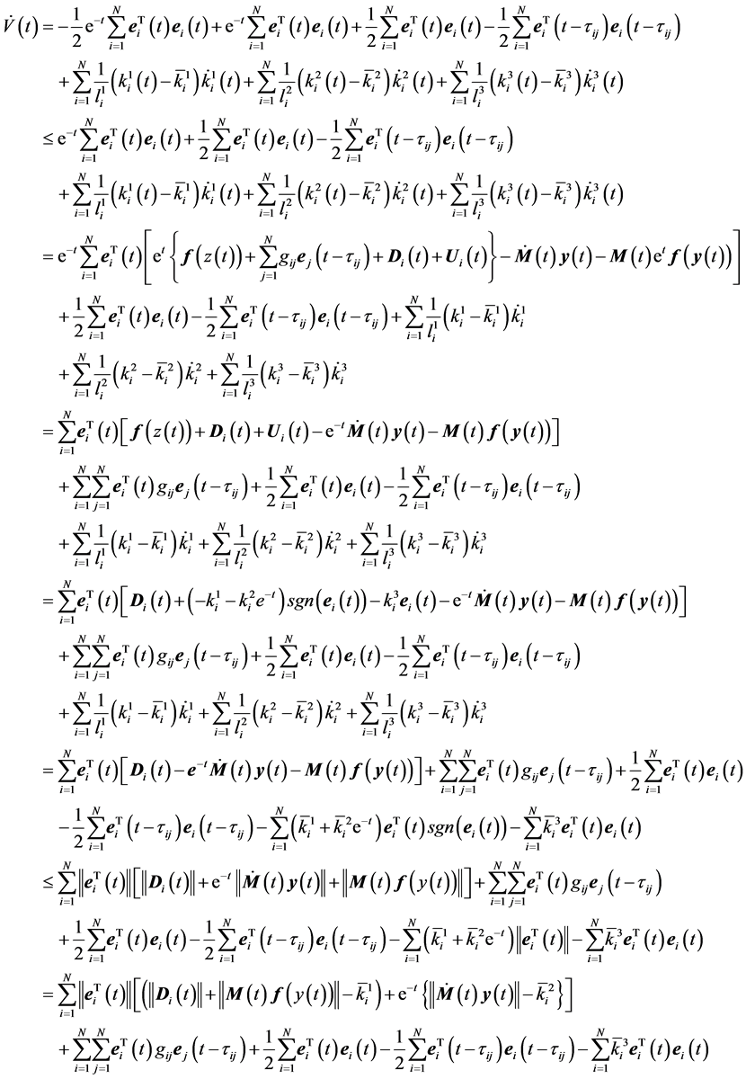
The time derivative of V(t) along the trajectories of system (3.6) is

(3.8)

Because chaos systems and the scaling function are bounded, $y\left(t\right)$ and ${\alpha }_i\left(t\right)$ are bounded. Furthermore, $f$ is a continuously vector function, there exists a positive constants $M_1$ satisfying $\Vert M\left(t\right)f\left(y\left(t\right)\right)\Vert \le M_1$ . Because Assumption 1 holds, there exists a positive constant $M_1$ satisfying $\Vert \stackrel{\dot{}}{M}\left(t\right)y\left(t\right)\Vert \le M_2$ . Because Assumption 2 holds, there exists a positive constant $d_i^{\mathrm{<mo>\; *\; </mo>}}$ satisfying $\Vert D_i\left(t\right)\Vert \le d_i^{\mathrm{<mo>\; *\; </mo>}}\left(i=\mathrm{1,2,}\cdots \mathrm{,}N\right)$ :

$\begin{array}{c}\stackrel{\dot{}}{V}\left(t\right)\le {\displaystyle \underset{i=1}{\overset{N}{\sum }}}\Vert e_i^{\text{T}}\left(t\right)\Vert \left[d_i^{*}-k_i^1-k_i^2{\text{e}}^{-t}+M_1+M_2{\text{e}}^{-t}\right]-{\displaystyle \underset{i=1}{\overset{N}{\sum }}}{k}_i^3{e}_i^{\text{T}}\left(t\right)e_i\left(t\right)\\ +{\displaystyle \underset{i=1}{\overset{N}{\sum }}}{\displaystyle \underset{j=1}{\overset{N}{\sum }}}{e}_i^{\text{T}}\left(t\right)g_{ij}{e}_j\left(t-{\tau }_{ij}\right)+\frac{1}{2}{\displaystyle \underset{i=1}{\overset{N}{\sum }}}{e}_i^{\text{T}}\left(t\right)e_i\left(t\right)-\frac{1}{2}{\displaystyle \underset{i=1}{\overset{N}{\sum }}}{e}_i^{\text{T}}\left(t-{\tau }_{ij}\right)e_i\left(t-{\tau }_{ij}\right)\\ ={\displaystyle \underset{i=1}{\overset{N}{\sum }}}\Vert e_i^{\text{T}}\left(t\right)\Vert \left[\left(d_i^{*}+M_1-k_i^1\right)+\left(M_2-k_i^2\right){\text{e}}^{-t}\right]-{\displaystyle \underset{i=1}{\overset{N}{\sum }}}{k}_i^3{e}_i^{\text{T}}\left(t\right)e_i\left(t\right)\\ +{\displaystyle \underset{i=1}{\overset{N}{\sum }}}{\displaystyle \underset{j=1}{\overset{N}{\sum }}}{e}_i^{\text{T}}\left(t\right)g_{ij}{e}_j\left(t-{\tau }_{ij}\right)+\frac{1}{2}{\displaystyle \underset{i=1}{\overset{N}{\sum }}}{e}_i^{\text{T}}\left(t\right)e_i\left(t\right)-\frac{1}{2}{\displaystyle \underset{i=1}{\overset{N}{\sum }}}{e}_i^{\text{T}}\left(t-{\tau }_{ij}\right)e_i\left(t-{\tau }_{ij}\right)\end{array}$ (3.9)

Tanking $k_i^1\ge d_i^{\mathrm{<mo>\; *\; </mo>}}+M_1$ and $k_i^2\ge M_2$ , $i=1,2,\cdots ,N$ , we obtain

$\begin{array}{c}\stackrel{\dot{}}{V}\left(t\right)\le -k^3{\displaystyle \underset{i\mathrm{<mo>\; =\; </mo>1}}{\overset{N}{\sum }}}{e}_i^{\text{T}}\left(t\right)e_i\left(t\right)+{\displaystyle \underset{i=1}{\overset{N}{\sum }}}{\displaystyle \underset{j=1}{\overset{N}{\sum }}}{e}_i^{\text{T}}\left(t\right)g_{ij}{e}_j\left(t-{\tau }_{ij}\right)\\ +\frac{1}{2}{\displaystyle \underset{i=1}{\overset{N}{\sum }}}{e}_i^{\text{T}}\left(t\right)e_i\left(t\right)-\frac{1}{2}{\displaystyle \underset{i=1}{\overset{N}{\sum }}}{e}_i^{\text{T}}\left(t-{\tau }_{ij}\right)e_i\left(t-{\tau }_{ij}\right)\end{array}$ (3.10)

where $k^3=\min \left(k_1^3,k_2^3,\cdots ,k_N^3\right)$ .

Let $e\left(t\right)={\left(e_1^{\text{T}}\left(t\right),e_2^{\text{T}}\left(t\right),\cdots ,e_N^{\text{T}}\left(t\right)\right)}^{\text{T}}\in R^{nN}$ . Then by Lemma 1, we have

$\begin{array}{c}\stackrel{\dot{}}{V}\left(t\right)\le -k^3{e}^{\text{T}}\left(t\right)e\left(t\right)+e^{\text{T}}\left(t\right)Qe\left(t-{\tau }_{ij}\right)\\ +\frac{1}{2}{e}^{\text{T}}\left(t\right)e\left(t\right)-\frac{1}{2}{e}^{\text{T}}\left(t-{\tau }_{ij}\right)e\left(t-{\tau }_{ij}\right)\\ \le -k^3{e}^{\text{T}}\left(t\right)e\left(t\right)+\frac{1}{2}{e}^{\text{T}}\left(t\right)Q{Q}^{\text{T}}e\left(t\right)+\frac{1}{2}{e}^{\text{T}}\left(t\right)e\left(t\right)\\ \le \left[-k^3+{\lambda }_{\max }\left(\frac{Q{Q}^{\text{T}}}{2}\right)+\frac{1}{2}\right]e^{\text{T}}\left(t\right)e\left(t\right)\end{array}$ (3.11)

Taking $k^3\ge {\lambda }_{\max }\left(\frac{Q{Q}^{\text{T}}}{2}\right)+\frac{1}{2}$ , we obtain

$\begin{array}{l}\stackrel{\dot{}}{V}\left(t\right)\le 0.\hfill \end{array}$ (3.12)

According to the Lyapunov stability theory, the error system (3.6) is asymptotically stable. This completes the proof.

Corollary 1. Suppose Assumptions 1 hold. For a given synchronization scaling function matrix $M\left(t\right)$ , if there exist positive constants $k_i^1$ , $k_i^2$ , $k_i^3$ ,

which satisfy $k_i^1\ge M_1$ , $k_i^2\ge M_2$ and $k_i^3\ge {\lambda }_{\max }\left(\frac{Q{Q}^{\text{T}}}{2}\right)+\frac{1}{2}$ , CDNs without

disturbance (3.1) can realize modified function projective synchronization via the control law :

#Math_111# (3.13)

where $sgn(\cdot )$ denotes the sign function.

By Theorem 1, it is easy to see that a similar proof holds for $D_i\left(t\right)=0\left(i=1,2,\cdots ,N\right)$ . Thus, the proof is omitted here.

Though the proposed error feedback control method is very simple, Choosing the appropriate feedback gains $k_i^1$ , $k_i^2$ and $k_i^3$ is still difficult. Thus, finding appropriate gains $k_i^1$ , $k_i^2$ and $k_i^3$ to achieve synchronization is still a challenging problem. In the following, an adaptive scheme is established in order to select the appropriate gains $k_i^1$ , $k_i^2$ and $k_i^3$ to realize MFPS in CDNs with or without disturbances.

Theorem 2. Suppose Assumptions 1 and 2 hold. For a given synchronization scaling function matrix $M\left(t\right)$ , CDNs with disturbance (3.2) can realize modified function projective synchronization via the control law :

$U_i\left(t\right)=-f\left(y_i\left(t\right)\right)+\left(-k_i^1\left(t\right)-k_i^2\left(t\right)e^{-t}\right)sgn\left(e_i\left(t\right)\right)-k_i^3\left(t\right)e_i\left(t\right)\mathrm{,}i=\mathrm{1,2,}\cdots \mathrm{,}N\mathrm{,}$ (3.14)

${\stackrel{\dot{}}{k}}_i^1\left(t\right)=l_i^1{e}_i^{\text{T}}\left(t\right)sgn\left(e_i\left(t\right)\right)\mathrm{,}i=\mathrm{1,2,}\cdots \mathrm{,}N\mathrm{,}$ (3.15)

${\stackrel{\dot{}}{k}}_i^2\left(t\right)=l_i^2{\text{e}}^{-t}{e}_i^{\text{T}}\left(t\right)sgn\left(e_i\left(t\right)\right)\mathrm{,}i=\mathrm{1,2,}\cdots \mathrm{,}N\mathrm{,}$ (3.16)

${\stackrel{\dot{}}{k}}_i^3\left(t\right)=l_i^3{e}_i^{\text{T}}\left(t\right)e_i\left(t\right)\mathrm{,}i=\mathrm{1,2,}\cdots \mathrm{,}N\mathrm{,}$ (3.17)

where $sgn(\cdot )$ denotes the sign function. $l_i^1>0,l_i^2>0$ and $l_i^3>0$ are arbi- trary positive constants. Proof. Construct the Lyapunov function

$\begin{array}{c}V\left(t\right)=\frac{1}{2}{\text{e}}^{-t}{\displaystyle \underset{i=1}{\overset{N}{\sum }}}{e}_i^{\text{T}}\left(t\right)e_i\left(t\right)+\frac{1}{2}{\displaystyle {\int }_{t-{\tau }_{ij}}^t}{\displaystyle \underset{i=1}{\overset{N}{\sum }}}{e}_i^{\text{T}}\left(v\right)e_i\left(v\right)\text{d}v+\frac{1}{2}{\displaystyle \underset{i=1}{\overset{N}{\sum }}}\frac{1}{l_i^1}{\left(k_i^1\left(t\right)-{\bar{k}}_i^1\right)}^2\\ +\frac{1}{2}{\displaystyle \underset{i=1}{\overset{N}{\sum }}}\frac{1}{l_i^2}{\left(k_i^2\left(t\right)-{\bar{k}}_i^2\right)}^2+\frac{1}{2}{\displaystyle \underset{i=1}{\overset{N}{\sum }}}\frac{1}{l_i^3}{\left(k_i^3\left(t\right)-{\bar{k}}_i^3\right)}^2,\end{array}$ (3.18)

The time derivative of V(t) along the trajectories of (3.6) is

(3.19)

Because chaos systems and the scaling function are bounded, $y\left(t\right)$ and ${\alpha }_i\left(t\right)$ are bounded. Furthermore, $f$ is a continuously vector function, there exists a positive constants $M_1$ satisfying $\Vert M\left(t\right)f\left(y\left(t\right)\right)\Vert \le M_1$ . Because As- sumption 1 holds, there exists a positive constant $M_2$ satisfying $\Vert \stackrel{\dot{}}{M}\left(t\right)y\left(t\right)\Vert \le M_2$ . Because Assumption 2 holds, there exists a positive constant $d_i^{\mathrm{<mo>\; *\; </mo>}}$ satisfying $\Vert D_i\left(t\right)\Vert \le d_i^{*}\left(i=1,2,\cdots ,N\right)$ :

$\begin{array}{c}\stackrel{\dot{}}{V}\left(t\right)\le {\displaystyle \underset{i=1}{\overset{N}{\sum }}}\Vert e_i^{\text{T}}\left(t\right)\Vert \left[\left(d_i^{*}+M_1-{\bar{k}}_i^1\right)+{\text{e}}^{-t}\left(M_2-{\bar{k}}_i^2\right)\right]\\ +{\displaystyle \underset{i=1}{\overset{N}{\sum }}}{\displaystyle \underset{j=1}{\overset{N}{\sum }}}{e}_i^{\text{T}}\left(t\right)g_{ij}{e}_j\left(t-{\tau }_{ij}\right)+\frac{1}{2}{\displaystyle \underset{i=1}{\overset{N}{\sum }}}{e}_i^{\text{T}}\left(t\right)e_i\left(t\right)\\ -\frac{1}{2}{\displaystyle \underset{i=1}{\overset{N}{\sum }}}{e}_i^{\text{T}}\left(t-{\tau }_{ij}\right)e_i\left(t-{\tau }_{ij}\right)-{\displaystyle \underset{i=1}{\overset{N}{\sum }}}{\bar{k}}_i^3{e}_i^{\text{T}}\left(t\right)e_i\left(t\right)\end{array}$ (3.20)

Tanking ${\bar{k}}_i^1\ge d_i^{\mathrm{<mo>\; *\; </mo>}}+M_1$ and ${\bar{k}}_i^2\ge M_2$ , $i\mathrm{<mo>\; =\; </mo>1,2,}\cdots \mathrm{,}N$ , we obtain

$\begin{array}{c}\stackrel{\dot{}}{V}\left(t\right)\le {\displaystyle \underset{i=1}{\overset{N}{\sum }}}{\displaystyle \underset{j=1}{\overset{N}{\sum }}}{e}_i^{\text{T}}\left(t\right)g_{ij}{e}_j\left(t-{\tau }_{ij}\right)+\frac{1}{2}{\displaystyle \underset{i=1}{\overset{N}{\sum }}}{e}_i^{\text{T}}\left(t\right)e_i\left(t\right)\\ -\frac{1}{2}{\displaystyle \underset{i=1}{\overset{N}{\sum }}}{e}_i^{\text{T}}\left(t-{\tau }_{ij}\right)e_i\left(t-{\tau }_{ij}\right)-{\bar{k}}^3{\displaystyle \underset{i=1}{\overset{N}{\sum }}}{e}_i^{\text{T}}\left(t\right)e_i\left(t\right)\end{array}$ (3.21)

where ${\bar{k}}^3=\min \left({\bar{k}}_1^3,{\bar{k}}_2^3,\cdots ,{\bar{k}}_N^3\right)$ .

Let $e\left(t\right)={\left(e_1^{\text{T}}\left(t\right),e_2^{\text{T}}\left(t\right),\cdots ,e_N^{\text{T}}\left(t\right)\right)}^{\text{T}}\in R^{nN}$ . Then by Lemma 1, we have

$\begin{array}{c}\stackrel{\dot{}}{V}\left(t\right)\le e^{\text{T}}\left(t\right)Qe\left(t-{\tau }_{ij}\right)+\frac{1}{2}{e}^{\text{T}}\left(t\right)e\left(t\right)\\ -\frac{1}{2}{e}^{\text{T}}\left(t-{\tau }_{ij}\right)e\left(t-{\tau }_{ij}\right)-{\bar{k}}^3{e}^{\text{T}}\left(t\right)e\left(t\right)\\ \le \frac{1}{2}{e}^{\text{T}}\left(t\right)\left(Q{Q}^{\text{T}}\right)e\left(t\right)+\frac{1}{2}{e}^{\text{T}}\left(t\right)e\left(t\right)-{\bar{k}}^3{e}^{\text{T}}\left(t\right)e\left(t\right)\\ \le \left[{\lambda }_{\max }\left(\frac{Q{Q}^{\text{T}}}{2}\right)+\frac{1}{2}-{\bar{k}}^3\right]e^{\text{T}}\left(t\right)e\left(t\right)\end{array}$ (3.22)

Taking ${\bar{k}}^3={\lambda }_{\max }\left(\frac{Q{Q}^{\text{T}}}{2}\right)+\frac{3}{2}$ , we obtain

$\begin{array}{l}\stackrel{\dot{}}{V}\left(t\right)\le -e^{\text{T}}\left(t\right)e\left(t\right).\hfill \end{array}$ (3.23)

According to the Lyapunov stability theory, the error system (3.6) is asymptotically stable. This completes the proof.

Corollary 2. Suppose Assumptions 1 hold. For a given synchronization scaling function matrix $M\left(t\right)$ , CDNs without disturbance (3.1) can realize modified function projective synchronization via the control law (3.14)-(3.17).

By Theorem 2, it is easy to see that a similar proof holds for $D_i\left(t\right)=0\left(i=1,2,\cdots ,N\right)$ . Thus, the proof is omitted here.

4. Computer Simulation

In this section, the chaotic Lorenz system is taken as nodes of CDNs to verify the effectiveness of the proposed scheme in Corollary 2.

Consider the following single Lorenz system:

$\{\begin{array}{l}{\stackrel{\dot{}}{x}}_1=a\left(x_2-x_1\right)\\ {\stackrel{\dot{}}{x}}_2=\left(b-x_3\right)x_1-x_2\\ {\stackrel{\dot{}}{x}}_3=x_1{x}_2-c{x}_3\end{array}$ (4.1)

where $a=10,b=28,c=\frac{8}{3}$ . Figure 1 and Figure 2 depict the chaotic attractor

and components of the Lorenz system respectively. The coupling configuration matrix $G=\left(g_{ij}\right)$ is chosen to be

Figure 1. Chaotic attractor of the Lorenz system.

Figure 2. Components of the Lorenz system.

$G=\left[\begin{array}{ccc}-1& 0& 1\\ 1& -1& 0\\ 0& 1& -1\end{array}\right]$

Complex networks with proportional delays can be described as follows:

$\left(\begin{array}{c}{\stackrel{\dot{}}{x}}_{i1}\left(t\right)\\ {\stackrel{\dot{}}{x}}_{i2}\left(t\right)\\ {\stackrel{\dot{}}{x}}_{i3}\left(t\right)\end{array}\right)=\left(\begin{array}{c}10\left(x_{i2}\left(t\right)-x_{i1}\left(t\right)\right)\\ \left(28-x_{i3}\left(t\right)\right)x_{i1}\left(t\right)-x_{i2}\left(t\right)\\ x_{i1}\left(t\right)x_{i2}\left(t\right)-\frac{8}{3}{x}_{i3}\left(t\right)\end{array}\right)+{\displaystyle \underset{j=1}{\overset{3}{\sum }}}{g}_{ij}{x}_j\left(q_{ij}t\right)+u_i\left(t\right),i=1,2,3$ (4.2)

where the controllers $u_i\left(t\right)$ satisfied: $U_i\left(t\right)=u_i\left({\text{e}}^t\right)$ , $U_i\left(t\right)$ can be designed by using Theorem 2 as follows:

$U_i\left(t\right)=-\left(\begin{array}{c}10\left(y_{i2}\left(t\right)-y_{i1}\left(t\right)\right)\\ \left(28-y_{i3}\left(t\right)\right)y_{i1}\left(t\right)-y_{i2}\left(t\right)\\ y_{i1}\left(t\right)y_{i2}\left(t\right)-\frac{8}{3}{y}_{i3}\left(t\right)\end{array}\right)+\left(-k_i^1\left(t\right)-k_i^2\left(t\right){\text{e}}^t\right)\left(\begin{array}{c}sgn\left(e_{i1}\left(t\right)\right)\\ sgn\left(e_{i2}\left(t\right)\right)\\ sgn\left(e_{i3}\left(t\right)\right)\end{array}\right)-k_i^3\left(t\right)\left(\begin{array}{c}{e}_{i1}\left(t\right)\\ e_{i2}\left(t\right)\\ e_{i3}\left(t\right)\end{array}\right)$

with

$\begin{array}{l}{\stackrel{\dot{}}{k}}_i^1\left(t\right)=l_i^1{\displaystyle \underset{j=1}{\overset{3}{\sum }}}{e}_{ij}\left(t\right)sgn\left(e_{ij}\left(t\right)\right)\\ {\stackrel{\dot{}}{k}}_i^2\left(t\right)=l_i^2{\text{e}}^t{\displaystyle \underset{j=1}{\overset{3}{\sum }}}{e}_{ij}\left(t\right)sgn\left(e_{ij}\left(t\right)\right)\\ {\stackrel{\dot{}}{k}}_i^3\left(t\right)=l_i^3{\displaystyle \underset{j=1}{\overset{3}{\sum }}}{e}_{ij}^2\left(t\right)\end{array}$

where $y_i\left(t\right)=x_i\left({\text{e}}^t\right)$ , $e_i\left(t\right)=y_i\left(t\right)-M\left(t\right)y\left(t\right)$ , $i=1,2,3.$

In this numerical simulation, we take the initial states as $x_1\left(0\right)={\left[34-4\right]}^{\text{T}}$ , $x_2\left(0\right)={\left[41-4\right]}^{\text{T}}$ , $x_3\left(0\right)={\left[-205\right]}^{\text{T}}$ , $x\left(0\right)={\left[5-35\right]}^{\text{T}}$ . We take $k_1^1\left(0\right)=1$ , $k_2^1\left(0\right)=2$ , $k_3^1\left(0\right)=3$ , $k_1^2\left(0\right)=4$ , $k_2^2\left(0\right)=5$ , $k_3^2\left(0\right)=6$ , $k_1^3\left(0\right)=12$ , $k_2^3\left(0\right)=15$ , $k_3^3\left(0\right)=16$ , $k_3^3\left(0\right)=16$ and

$M\left(t\right)=diag\left(4+\sin \frac{2\text{π}t}{10},4+\cos \frac{2\text{π}t}{10},4+\sin \frac{2\text{π}t}{10}\right)$ . The numerical results are

presented in Figure 3 and Figure 4. Figure 3 displays the state phases of the Lorenz system. The time evolution of the synchronization errors is depicted in Figure 4, which displays $e\left(t\right)\to 0$ with $t\to \infty$ . These results show that function projective synchronization takes place with the desired scaling function in complex networks (4.2).

5. Concluding Remarks

In this paper, function projective synchronization schemes for complex net- works with proportional delays are given by a error feedback control method. Numerical simulation is provided to show the effectiveness of our result.

Figure 3. State phases of the Lorenz system.

Figure 4. The time evolution of the synchronization errors e.

Acknowledgements

This work is jointly supported by the Natural Science Foundation of China (11101187, 61573005, 11361010), the Scientific Research Fund of Fujian Provincial Education Department of China (JAT160691).

Conflicts of Interest

The authors declare no conflicts of interest.

References

[1]	Ott, E., Grebogi, C. and Yorke, J.A. (1990) Controlling Chaos. Physical Review Letters, 11, 1196-1199. https://doi.org/10.1103/PhysRevLett.64.1196
[2]	Gang, H. and Qu, Z.L. (1994) Controlling Spatiotemporal Chaos in Coupled Map Lattice Systems. Physics Letters A, 72, 68-73. https://doi.org/10.1103/PhysRevLett.72.68
[3]	Carroll, T.L. and Pecora, L.M. (1990) Synchronization in Chaotic Systems. Physical Review Letters, 64, 821-824. https://doi.org/10.1103/PhysRevLett.64.821
[4]	Yang, T. (2004) A Survey of Chaotic Secure Communication Systems. International Journal of Computational Vision and Robotics, 2, 81-130.
[5]	Lu, J.Q. and Cao, J.D. (2005) Adaptive Complete Synchronization of Two Identical or Different Chaotic (Hyperchaotic) Systems with Fully Unknown Parameters. Chaos, 15, 4-9. https://doi.org/10.1063/1.2089207
[6]	Wang, T., Li, T., Yang, X., Fei, S. (2012) Cluster Synchronization for Delayed Lur’e Dynamical Networks Based on Pinning Control. Neurocomputing, 83, 72-82.
[7]	Shahverdiev, E.M. and Sivaprakasam, S. (2002) Lag Synchronization in Time Delayed Systems. Physics Letters A, 292, 320-324. https://doi.org/10.1016/S0375-9601(01)00824-6
[8]	Rulkov, N.F., Sushchik, M.M. and Tsimring, L.S., et al. (1995) Generalized Synchronization of Chaotic Oscillators. Physical Review Letters, 51, 980-994.
[9]	Wang, L., Qian, W. and Wang, Q. (2015) Bounded Synchronization of a Time Varying Dynamical Network with Nonidentical Nodes. International Journal of Systems Science, 46, 1-12. https://doi.org/10.1080/00207721.2013.815825
[10]	Rosenblum, M.G., Pikovsky, A.S. and Kurths, J. (1996) Phase Synchronization of Chaos in Directionally Coupled Chaotic Systems. Physical Review Letters, 761, 804-807.
[11]	Kim, C., Rim, S., Kye, W., Yu, J.R. and Park, Y. (2003) Anti-Synchronization of Chaotic Oscillators. Physics Letters A, 320, 39-46. https://doi.org/10.1016/j.physleta.2003.10.051
[12]	Mainieri, R. and Rehacek, J. (1999) Projective Synchronization in Three-Dimensional Chaotic Systems. Physical Review Letters, 82, 3042-3045.
[13]	Tang, X., Lu, J. and Zhang, W. (2007) The FPS of Chaotic System Using Backstepping Design. International Journal of Dynamics and Control, 5, 216-219.
[14]	Chen, Y. and Li, X. (2009) Function Projective Synchronization between Two Identical Chaotic System. Chaos, Solitons & Fractals, 42, 2399-2402. https://doi.org/10.1016/j.chaos.2009.03.120
[15]	Du, H., Zeng, Q. and Wang, C. (2010) Modified Function Projective Synchronization of Chaotic Systems. Nonlinear Analysis: Real World Applications, 11, 705-712.
[16]	Park, J., Lee, J. and Won, S. (2013) Modified Function Projective Synchronization for Two Different Chaotic Systems Using Adaptive Fuzzy Nonsingular Terminal Sliding Mode Control. 13th International Conference on Control, Automation and Systems, Gwangju, 20-23 October 2013, 28-33. https://doi.org/10.1109/iccas.2013.6703858
[17]	Li, J. and Li, N. (2011) Modified Function Projective Synchronization of a Class of Chaotic Systems. Acta Physica Sinica, 60, 147-149.
[18]	Wei, D., Hong, W., et al. (2013) Modified Function Projective Synchronization of a Classic Chaotic Systems with Unknown Disturbances Based on Adaptive Integral Sliding Mode Control. 2013 Fourth International Conference on Intelligent Systems Design and Engineering Applications, Gwangju, 6-7 November 2013, 382-385.
[19]	Feng, M. (2013) Adaptive Modified Function Projective Synchronization for Complex Four-Dimensional Chaotic Systems. Proceedings of 2013 International Conference on Computing, Networking and Communications, Honolulu, 3-6 February 2013, 1537-1541.
[20]	Du, H., Lu, N. and Li, F. (2012) Modified Function Projective Synchronization of Two Different Chaotic Systems with Parameter Perturbations. Proceedings of 2012 International Conference on Measurement, Information and Control, Harbin, 18-20 May 2012, 761-764.
[21]	Lu, J. and Cao, J. (2009) Synchronization-Based Approach for Parameters Identification in Delayed Chaotic Neural Networks. Physics Letters A, 382, 672-682.