Identification and Interpretation of Earth’s Atmosphere Dynamics’ and Thermodynamics’ Similarities between Rogue Waves and Oceans’ Surface Geostrophic Wind ()
Received 19 February 2016; accepted 8 April 2016; published 11 April 2016

1. Introduction
Scientists interested in weather climate make extensive use of the geostrophic wind behavior in their practices to explain many meteorological phenomena such as the direction of the winds that take place around the low pressure systems. The questioning that faces the public interested in information disseminated by meteorologists is to know exactly what means the geostrophic wind. Besides the poor phenomenological definitions scattered in very little scientific work, there is unfortunately no book which gives importance to the algebraic definition of the geostrophic wind. E.g., according to most observers, the reasons why the geostrophic wind is parallel to the isobars are not explained by a relevant theory. Teaching those who study the earth’s atmosphere physics that the geostrophic wind leaves depressions on the left in the northern hemisphere (or on the right in the southern hemisphere) without providing any mathematical formula that consolidates these very useful laws, is the same think as preaching in the desert. Efforts will be made in our work so that many well known laws set without proper mathematical formula will be explained, as simple as possible, accordingly to relevant demonstrations. Our approach has the biggest advantage of highlighting all the relevant characteristics of geostrophic wind (e.g., geostrophic wind’s characteristics already known to the public and its specifics completely unknown even by specialists in meteorology). In this paper, we also want to show that, due to very strong surface winds that accompany them, tornadoes occur in a lying on the ground’s surface deep column in which the geostrophic balance settles. Undoubtedly, identification and interpretation of earth’s atmosphere dynamics’ and thermody- namics’ similarities between rogue waves and oceans’ surface geostrophic wind will be an easy exercise to researchers who will give importance to result provided by our paper.
2. The Geostrophic Wind in Rectangular Coordinates
2.1. Forces of Significance in Atmospheric Motion
2.1.1. Gravity Force in Spherical Approximation
Since meteorology is dealing with the masses in the vicinity of the earth, we shall consider the mass of the earth (Me) and any other mass (m). For the time being we shall neglect the fact that the earth is rotating. Moreover, we shall assume that the earth is a homogeneous sphere with its center of mass at its geometrical center, so that we can chose the earth’s center as the origin of a coordinate system. The assumption of homogeneity is a good assumption for most meteorological requirements. Suppose a point P is located at distance OP = r from the center of the spherical earth, as shown in Figure 1. The location of P with respect to the earth’s center is given by the position vector . A mass m located at P is subject to the force of gravitation
  of magnitude
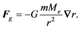
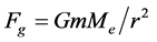 . This force (Figure 1) accelerates the mass toward the earth, and the acceleration vector, or the force of gravitation is
 (1)
(1)
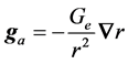
Since the acceleration is directed opposite to the unit vector , we usually deal with unit mass, so that m = 1 and we write the force of gravitation for unit mass in the form
 (2)
(2)
 is called the earth’s gravitational constant. Numerical values of the pertinent constant are

2.1.2. Frictional Forces/Pressure Forces
Frictional forces (Figure 2) act on the surface of a fluid volume. They are stresses. There are normal stresses and tangential stresses. If the fluid is completely at rest, all tangential stresses must vanish, and only normal stresses can remain (this fact distinguishes fluids from solids, because solids can remain at rest when they are subject to tangential stresses). Thus, in a state of rest or equilibrium, the normal stresses must be defined in such a way they reduce to the hydrostatic pressure when the fluid is at rest. The magnitude of viscous frictional force, F, is
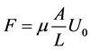 (3)
(3)
where  is the viscosity of the fluid and (A) the acting area. Resulting component of frictional force along the xyz-axis are well explained in [1] - [4] .
Whether hydrostatic or not, the pressure is defined as force per unit area. Accordingly, the pressure force P is equal to pressure time’s area. We shall treat the pressure as hydrostatic and as a normal stress [4] .
2.1.3. Coriolis Force per Unit Mass
According to the meteorological rectangular coordinates rotating frame (Figure 3).
Components of the earth’s rotation vector ( ) in meteorological rectangular frame (Figure 3) are
1) In the Northern Hemisphere
 (4)
(4)
![]()
Figure 1. The mass (m) located at P is subject to the force of gravitation, directed as shown in the figure.
![]()
Figure 2. Couette’s proofs of frictional forces existences (the frictional forces are retarding forces).
![]()
Figure 3. Meteorological rectangular coordinates rotating frame.
Hence: the N-H Coriolis force per unit mass
![]() (5)
(5)
2) In the Southern Hemisphere
![]() (6)
(6)
Hence: the S-H Coriolis force per unit mass
![]() (7)
(7)
where (u, v, w) are the components in meteorological rectangular frame of the relative velocity. Coriolis force is apparent force and not real force as the force of gravitation or pressure force. This apparent force arises purely from the fact that the motion is observed from a rotating frame of reference. Nevertheless, this force is very real to the rotating observer.
2.2. Equation of Relative Motion in Rectangular Coordinates
The equation of relative motion in rectangular coordinates is
![]() (8)
(8)
The symbol ![]() denotes the relative velocity, i.e., the velocity relative to a point which is fixed with respect to the surface of the earth. The accelerations and forces are (all per unit mass).
denotes the relative velocity, i.e., the velocity relative to a point which is fixed with respect to the surface of the earth. The accelerations and forces are (all per unit mass).
![]() = relative acceleration.
= relative acceleration.
![]() = pressure gradient force.
= pressure gradient force.
![]() = Coriolis force.
= Coriolis force.
![]() = force of gravity.
= force of gravity.
![]() = “frictional” force.
= “frictional” force.
Meteorologists have at least an intuitive feeling that fluid flow is somehow related to the mass distribution of the fluid. However, there is no equation in all of fluid dynamics which would allow us to infer the velocity field given knowledge of the mass field. All we can infer are time-rates-of-change of the velocity field, i.e., accelerations. We have already seen [4] that molecular frictional forces can be neglected for most purposes in the free atmosphere. The question now arises: are there situations where some of the remaining forces in the equation of motion are negligible? The answer to this question is “yes”, and we shall now discuss one very important case: the geostrophic wind (or geostrophic balance).
2.3. The Geostrophic Balance Equation
The situation where some of the remaining forces of Equation (8) are negligible can be described by (Equation (9)) called the geostrophic balance equation
![]() (9)
(9)
in which relative acceleration and frictional force are negligible compared to pressure, Coriolis and gravitation force.
2.4. The Geostrophic Wind in Rectangular Coordinates
Using vector product (symbol![]() ), we can transform Equation (9) and write (9-a)
), we can transform Equation (9) and write (9-a)
![]() (9-a)
(9-a)
In the goal to obtain (9-b)
![]() (9-b)
(9-b)
where: ![]() is perpendicular to the horizontal pressure gradient vector,
is perpendicular to the horizontal pressure gradient vector, ![]() is
is ![]() unit vector, and
unit vector, and ![]() in the case of the phenomenological definition of geostrophic wind.
in the case of the phenomenological definition of geostrophic wind.
Hence:
The Geostrophic Vector (or Wind) in the Northern-Hemisphere
![]() (10)
(10)
The Geostrophic Vector (or Wind) in the Southern-Hemisphere
![]() (11)
(11)
3. Fundamentals of Geostrophic Wind Dynamics and Thermodynamics
Equations (10) and (11) lead to 06 geostrophic vector specifics (or fundamental properties):
P1: the geostrophic winds (as defined) are perpendicular to the horizontal pressure gradient vector.
P2: the geostrophic winds (as defined) are horizontal (they are perpendicular to![]() ).
).
P3: the geostrophic wind (as defined) is parallel (or tangent at any point) to the isobars.
Proof: along an isobar, ![]() is perpendicular to the elementary displacement
is perpendicular to the elementary displacement![]() . The mathematical reason is the fact that, along an isobar, p is a Constant. Therefore
. The mathematical reason is the fact that, along an isobar, p is a Constant. Therefore
![]() .
.
This allows stating P3.
P4: the geostrophic winds (as defined) are inversely proportional to![]() . Its magnitude is therefore able to dizzily increase close to the equator (where
. Its magnitude is therefore able to dizzily increase close to the equator (where ![]() tends to zero): Geostrophic winds are (as defined) more devastating in the tropics than in temperate or Polar Regions.
tends to zero): Geostrophic winds are (as defined) more devastating in the tropics than in temperate or Polar Regions.
P5: The geostrophic winds are (as defined) stronger when the density (r) of air decreases.
P6: the geostrophic winds (as defined) move leaving the low pressure to their left in the Northern Hemisphere. They move leaving the low pressure to their right in the Southern Hemisphere (Figure 4).
(This statement is provided by the properties of the vector product).
![]()
Figure 4. Geostrophic wind’s orientations (theoric and visual).
4. Horizontal Profiles of Tornadoes’ Winds
According to the Geostrophic Balance Equation (e.g., Equation (9)), if a wind (even a moderate one) blows on a Compilation of Highest Horizontal-Temperature-Gradients’ Systems (HHTGS) which means the Compilation of Highest Horizontal-Pressure-Gradients’ Systems (HHPGS), this wind will turn spontaneously geostrophic wind. In other words, it will trigger a tornado (in the case of the compilation of HHTGS triggered by hot thermal sources). It is this kind of shows that the Earth’s atmosphere has accustomed us (Figure 5). In the atmosphere, winds are random processes beyond expected. In fact, no climate model can predict its occurrence or its total dissipation. That totally unexpected nature of the winds, made the outbreak of tornadoes, something unpredictable. As indicated by many observers [5] - [18] , a total lack of wind frequently comes before the outbreak of either tornadoes or rogue waves. It is important to note that this total lack of wind leads to the installation of HHTGS which means (in gas like air) the installation of HHPGS triggered by hot thermal sources in its vicinity. It is now evident that Tornadoes’ winds are geostrophic winds.
5. Compelling Similarities between Ocean’s Surface Tornadoes and Rogue Waves
Tornadoes, as has been demonstrated in the preceding paragraphs, derive from upsurge of 02 meteorological events: the compilation of HHPGS triggered by a hot thermal source and the occurrence of Coriolis force triggered by the wind which blows in the vicinity of the “building” made of compilation of HHTGS (or HHPGS). If we agree to give the name “Epicenter” to the place where the local sea level pressure minimum appears, it will then be easy to point out parallels between solitary waves (Figure 6 [19] ) and thunderclouds accompanying Tornadoes that appear over land’s surface (Figure 5). Indeed, when the geostrophic balance appears above the
![]()
Figure 5. Tornadoes’ thundercloud and cloud-to-ground lightning flash.
![]()
Figure 6. Ocean’s surface solitary wave triggered by atmosphere lower boundary’s decreasing pressures [19] .
oceans, it triggers 02 spontaneous and simultaneous spectacular events: a Tornado and a solitary wave which peaks at the Epicenter of the horizontal low pressure systems. This solitary wave has the same life cycle that Tornado. The real nature of the physical processes behind the formation of rogue waves (e.g., rogue waves are solitary waves. They are worst nightmares of sailors traveling through the oceans because they are devastating and unpredictable) is well known now.
6. Conclusion
Our work shows once again that to better understand the behavior of natural phenomena, it is essential to combine the theories with based observations. Obviously, observations cannot be relevant without a theory that guides the observers. Conversely, no theory can be validated without experimental verification. Synoptic ob- servations show that in the “free atmosphere!” the wind vectors are very nearly parallel to isobars, and the flow is perpendicular to the horizontal pressure gradient force, at least at any given instant. This kind of information recommends great caution when making geostrophic approximations. Our work shows that for hurricanes and tornadoes, there is no need to move away from the surface of the ground to observe the geostrophic balance. This is not necessarily true when determining the direction of the winds around the low pressures systems using maps derived from the “ground based-pressures” (instead of: space based-pressures). Nearly parallel to isobars did not mean parallel to isobars. Since the geostrophic balance reaches the surface of the ground in the case of cyclones, horizontal profiles of wind associated to this weather event can be deduced from the 06 fundamental properties stated in this work. Our results will certainly help people who spend huge sums of money to run (sometimes taking considerable risks) after the spectacular thermodynamically shows offered by tornadoes.