A Two-Dimensional Mathematical Model to Analyze Thermal Variations in Skin and Subcutaneous Tissue Region of Human Limb during Surgical Wound Healing ()
Received 19 October 2015; accepted 2 February 2016; published 5 February 2016

1. Introduction
Enzymes play a key role in the healthy functioning of organs and glands of our body. They work properly in 20˚C - 37˚C body temperature [1] [2] . Any disturbance in body temperature disturbs the proper functioning of enzymes (metabolic activity). Thus it becomes important to study thermal variations in order to develop a mechanism for establishing the limits of thermal regulation in human body during the healing process.
Pennes [3] in 1948 first gave the well known bio-heat equation of heat transfer in perfused tissue for the analysis of temperatures in the resting human forearm. Perl [4] in 1962 used it to illustrate heat distribution and tissue blood flow in body tissues. Since then it has been used by many researchers and scientists [1] [5] - [11] for analysis in their respective areas of research. A lot of research on wound healing has also been done by considering different parameters like size and shape of the wound, the effect of growth factors, the effect of angiogenesis, the effect of oxygen concentration at the wound site etc. [12] - [18] . A few scientists have studied temperature variations caused due to wound healing process after surgery [1] [19] [20] .
In this paper, a two-dimensional finite element model has been developed for transient state temperature distribution in normal and operated peripheral tissues of human limb during healing time by using Pennes’ bio heat equation [3] . Assuming the cross section of human limb to be circular in shape, model has been developed in polar coordinates (r, θ). The effect of the density of blood vessels in different layers of dermal region on temperature distribution is incorporated by considering the physical and physiological parameters to be function of space coordinate “r” only in case of normal tissues and increasing function of time “t” also in case of abnormal tissues [1] [19] [20] . The position of major arteries, lying deep inside the skin, carrying blood from the core to the limbs is not symmetrically distributed along the angular direction [21] . Variable core temperature along angular direction “θ” [22] has been considered to incorporate the effect of position of major arteries in limbs. The outer surface is exposed to the environment and an appropriate boundary condition for heat loss at the outer surface has been incorporated.
2. Model Description
Nomenclature
2.1. Mathematical Formulation
Pennes’ bio-heat equation for two dimensional unsteady state case in polar coordinates takes the form:
 (1)
(1)
Here K, S, mb, cb, ρ, c, T and Tb are thermal conductivity, metabolic heat generation rate, rate of blood mass flow per unit volume, specific heat of blood, tissue density, specific heat of tissue, unknown tissue temperature and temperature of blood.
The inner core of the human limb is at a variable temperature and hence it is formulated as:
 (2)
(2)
Here R0 is the radius at the inner core of skin and  [6] is given by:
 (3)
(3)
where c1, c2, c3 are determined using conditions:
 (4)
(4)
Here  is greater than
 . The boundary condition at outer surface of skin is:
 (5)
(5)
Here h, Ta, L, E and  are heat transfer coefficient, atmospheric temperature, latent heat of vaporization,
rate of evaporation and partial derivative of unknown tissue temperature along the normal direction to the skin surface. Heat transfer along angular direction is assumed to be negligible.
The surface of the limb is insulated initially [1] [9] . So initial condition is given by:
 (6)
(6)
2.2. Use of Finite Element Method―Discretisation of Domain
The circular cross section of annular shaped region of peripheral tissues of human limb is discretised into a total of twenty four elements (Figure 1). Skin tissues are naturally divided into three layers viz. epidermis, dermis and subcutaneous tissues. We have further divided dermis into four layers. Each layer is further divided into four coaxial circular sectors at . Thus there are in all twenty four elements and twenty eight nodes. The bio heat equation can be written for each element in discretised variational form as:
 (7)
(7)
where Ω(e) and Γ(e) represents the domain and outer boundary along the angular direction of eth element. In the second integral λ(e) is 1 for surface elements and zero for other elements.
2.3. Physiological Parameters for Normal and Abnormal Tissues
In this model, it is assumed that there is negligible variation in thermal conductivity, blood mass flow rate and metabolic heat generation rate along angular direction.
![]()
Figure 1. Cross section of annular shaped region of peripheral tissues of human limb. In all there are twenty four coaxial circular sector elements and twenty eight nodes.
2.3.1. For Normal Tissues
There is no blood flow and metabolic heat generation in the epidermis. Hence it is assumed that M3 = 0 = S3 in epidermis. Physical and physiological parameters like thermal conductivity (K1), rate of heat transfer due to blood mass flow (M1) and metabolic heat generation rate (S1) have almost constant value in subcutaneous layer. In dermis K2, M2 and S2 are function of radial coordinate only and expressed by interpolating linearly between the corresponding values at epidermis and subcutaneous tissues.
 (8)
(8)
2.3.2. For Abnormal Tissues
Since surgery results in loss of blood and tissue, it is assumed that initially at time t = 0, blood mass flow rate and metabolic heat generation rate is almost negligible and gradually increase with time to attain normal values. For abnormal tissues these are increasing function of time too.
![]() (9)
(9)
Here
![]() (10)
(10)
where ![]() are unknown constants which are found using conditions [1] :
are unknown constants which are found using conditions [1] :
![]() (11)
(11)
2.4. Interpolation Function for Circular Coaxial Sector Element
We have chosen the bilinear shape function in polar coordinates for the variation of temperature within each element,
![]() (12)
(12)
Here
![]() (13)
(13)
Here i, j, k and l are the local node numbers. The interpolation functions, thus, obtained are―
![]() (14)
(14)
Here
![]() (15)
(15)
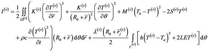
In this paper, the domain has been divided into circular coaxial sector elements of varying thickness i.e. “a” takes three different values: ![]() for subcutaneous tissues, dermis and epidermis respectively. Using the above values and expressions for physical and physiological parameters and expression for temperature variation (12) in (7), integral
for subcutaneous tissues, dermis and epidermis respectively. Using the above values and expressions for physical and physiological parameters and expression for temperature variation (12) in (7), integral ![]() is evaluated as:
is evaluated as:
![]() (16)
(16)
Equation (16) has been differentiated with respect to each nodal temperature of the element then expressed in matrix form and minimized. The corresponding global matrix equation has been formed and assembled. Crank Nicolson Technique has been employed to solve the system of equations to obtain the temperature profile at each node for progressive time. A computer program has been developed in MATLAB to simulate the results.
3. Numerical Results and Discussions
In order to enhance the applicability of the present model in different climatic conditions, the numerical calculations have been done for three cases of atmospheric temperatures. The values of physical and physiological parameters taken [1] [10] [19] [22] [23] to obtain the numerical results are given in Table 1 and Table 2.
![]()
Table 1. Value of physical and physiological parameters.
![]()
Table 2. Value of M1 and S1 at different Ta and E.
The constants ![]() have been assigned the following values:
have been assigned the following values:
![]()
Nodal temperature versus time graphs (Figures 2-8), steady state nodal temperature versus radial coordinate graphs (Figures 9-11) and steady state nodal temperature versus angular coordinate graphs (Figures 12-14) have been plotted for three different atmospheric temperatures for both, normal and abnormal tissues.
For plotting Figures 2-8 four nodes chosen are: one at core of the skin, one at the interface of subcutaneous and dermis, one at the interface of dermis and epidermis and one at the surface of the skin for each value of θ = 0(π/2)3π/2. For plotting Figures 9-11 seven nodes chosen are at ri, i = 0(1)6 for each value of θ = 0(π/2)3π/2. For plotting Figures 12-14 the five nodes chosen are at θ = 0, π/2, π, 3π/2 and 2π for each ri; i = 0, 1, 5 and 6. These graphs give us an idea about the magnitude of the thermal effect of surgical wound on temperature profiles in the skin layers.
Figure 2 represents thermal variations at selected nodes with progression of time for Ta = 15˚C and E = 0 gm/cm2 min. Similarly Figures 3-5 and Figures 6-8 represents thermal variations for Ta = 23˚C, E = 0.0(0.00024)0.00048 gm/cm2 min and Ta = 33˚C, E = 0.00024(0.00024)0.00072 gm/cm2∙min respectively. Figure 9 represents nodal temperature distribution (when thermal equilibrium is reached) with respect to radial coordinate at Ta = 15˚C and E = 0 gm/cm2 min. Likewise Figures 10(a)-(c) and Figures 11(a)-(c) represent steady state nodal temperature distribution for Ta = 23˚C, E = 0.0(0.00024)0.00048 gm/cm2 min and Ta = 33˚C, E = 0.00024(0.00024)0.00072 gm/cm2 min respectively. Figure 12, Figures 13(a)-(c) to Figures 14(a)-(c) represent steady state temperature distribution along angular direction for Ta = 15˚C, 23˚C (E = 0.0(0.00024)0.00048 gm/cm2∙min) and 33˚C (E = 0.00024(0.00024)0.00072 gm/cm2∙min) respectively.
All the graphs (Figures 2-14) show that at the skin core nodal temperatures are given by the function f(θ) as assumed.
From Figures 2-8 it is observed that with the increase in time, there is steep decrease in temperature for first 10 minutes and 20 minutes for normal and abnormal tissues respectively. This is due to the fact that on exposure to atmosphere (at lower temperature), heat is lost from the tissues due to radiation and conduction. Heat is also lost due to evaporation of sweat, which is produced on activation of sweat glands when peripheral tissues are at higher temperature. Heat of peripheral tissues is lost in the form of latent heat of vaporization. This fall in temperature is higher in abnormal tissues than that in the normal ones. It is because of temporary vasoconstriction in incised blood vessels of the tissues [2] [24] . Results show that, abnormal tissue temperature takes more time to obtain steady state than that of normal tissue. For normal tissues, the temperature becomes almost steady after
![]()
Figure 2. Graph between nodal temperature T and time t for normal (black solid line) and abnormal (blue solid line) tissues at (a) θ = 0, 2π, (b) θ = π/2, 3π/2, (c) θ = π, ![]() and
and![]() .
.
![]()
Figure 3. Graph between nodal temperature T and time t for normal (black solid line) and abnormal (blue solid line) tissues at (a) θ = 0, 2π, (b) θ = π/2, 3π/2, (c) θ = π, ![]() and
and![]() .
.
20 minutes. In case of abnormal tissues, after attaining the minimum value the temperature begins to rise for about 180 - 250 minutes without and with different rates of evaporation (Figures 2-8). It is further observed that during this increment period, the rate of increase in temperature is fast for first 40 - 50 minutes approximately followed by further increment but with slower rate in the remaining period. This may be due to the fact that initially the rate of blood mass flow and heat generated due to metabolic activity of the operated tissues are very small in comparison to normal tissues but as time progresses, the value of these parameters also increase which helps the abnormal tissue to return to normal temperature and restart cell mitotic division to accomplish wound healing [25] [26] . Thus abnormal tissues take more time to attain steady state temperature in comparison to normal tissues and it can be validated on the basis of experimental results of Gannon [26] .
In all the graphs, the fall in tissue temperature is more at the skin surface in comparison to the interior tissues because more heat is lost at the surface due to convection, radiation and evaporation.
![]()
Figure 4. Graph between nodal temperature T and time t for normal (black solid line) and abnormal (blue solid line) tissues at (a) θ = 0, 2π, (b) θ = π/2, 3π/2, (c) θ = π, ![]() and
and![]() .
.
![]()
Figure 5. Graph between nodal temperature T and time t for normal (black solid line) and abnormal (blue solid line) tissues at (a) θ = 0, 2π, (b) θ = π/2, 3π/2, (c) θ = π, ![]() and
and![]() .
.
For the same rates of evaporation, the decline in tissue temperature is more at lower atmospheric temperature than that at higher atmospheric temperature and the steady state temperature of the tissue at lower atmospheric temperature is less than that with the higher atmospheric temperature (Figure 2, Figure 3 or Figure 4, Figure 6 or Figure 5, Figure 7).This is because the temperature gradient at the skin surface is more at lower atmospheric temperature than that at higher atmospheric temperature and amount of heat transfer is directly proportional to temperature gradient. But with the slight increase in evaporation rate at higher atmospheric temperature, the temperature profiles become closer in spite of considerable amount of difference in atmospheric temperature. For example, it is observed that the temperature profiles for Ta = 15˚C and E = 0.0 gm/cm2 (Figure 2) and Ta = 33˚C, E = 0.24 × 10⁻³ gm/cm2 (Figure 6) are close in spite of a difference of 18˚C in atmospheric temperature and a small rate of sweat evaporation at higher temperature. This highlights the significant role of evaporation of sweat by utilizing latent heat of vaporization in gaining thermal balance.
![]()
Figure 6. Graph between nodal temperature T and time t for normal (black solid line) and abnormal (blue solid line) tissues at (a) θ = 0, 2π, (b) θ = π/2, 3π/2, (c) θ = π, ![]() and
and![]() .
.
![]()
Figure 7. Graph between nodal temperature T and time t for normal (black solid line) and abnormal (blue solid line) tissues at (a) θ = 0, 2π, (b) θ = π/2, 3π/2, (c) θ = π, ![]() and
and![]() .
.
For the same atmospheric temperature, the fall in tissue temperature increases as the rate of evaporation increases (Figures 3-5 or Figures 6-8).This again shows that rate of evaporation has a significant role in temperature regulation in SST region.
From Figures 9-11 it is observed that the slope of the curve changes at the junction of each layer (r = 2.5(0.1)2.9 cm). This is due to the different physiological properties of each layer. The steepness of the curves increases as we move from the inner core towards outer surface. It is because of the maximum temperature gradient at the surface which results in maximum temperature fall at the surface and this effect reduces as we move towards core of the limb. Also it is observed that at a given atmospheric temperature and evaporation rate, the thermal variation along angular direction decreases as we move radialy outwards from the core. It implies that effect of core temperature on thermal distribution of tissues decreases in angular direction with increase in distance from the core.
![]()
Figure 8. Graph between nodal temperature T and time t for normal (black solid line) and abnormal (blue solid line) tissues at (a) θ = 0, 2π, (b) θ = π/2, 3π/2, (c) θ = π, ![]() and
and![]() .
.
![]()
Figure 9. Nodal temperature versus distance from core graph for Ta = 15˚C, E = 0.0 gm/cm2∙min, η = ν = 0.01 for normal (black solid line) and abnormal (blue solid line) tissues at thermal equilibrium. Note: Nodal temperature of normal and abnormal tissues is almost same at equilibrium so overlapping of curves has occurred.
From Figure 12, Figures 13(a)-(c) and Figures 14(a)-(c) it is noted that the variation in tissues temperature in angular direction, in each layer reflects the effect of assumed boundary condition at the core of limb.
On comparing Figure 9 with Figure 10(a), Figure 10(b) with Figure 11(a), Figure 10(c) with Figure 11(b), it is observed again that (for fixed evaporation rate) the fall in nodal temperature along radial direction increases as atmospheric temperatures decreases but lowering of atmospheric temperature has no significant effect on the fall of nodal temperature along angular direction (compare Figure 12 with Figure 13(a), Figure 13(b) with Figure 14(a) and Figure 13(c) with Figure 14(b)). It is because lowering of atmospheric temperature is symmetric about “θ” and increases temperature gradient significantly in radial direction only.
On comparing Figures 10(a)-(c) or Figures 11(a)-(c), it is observed that at given atmospheric temperature, the increase in evaporation rate increases the decline in nodal temperature along radial direction but has no effect on the thermal variations along angular direction (compare Figures 13(a)-(c) or Figures 14(a)-(c)). It is because the increment in evaporation rate is also symmetric about “θ” and increases temperature gradient significantly in radial direction only.
The steady state nodal temperature (SSNT) values shown in Figures 2(a)-(c) can also be observed in Figure 9 for θ = 0 (or 2π), θ = π/2 (or 3π/2) and θ = π respectively. Further same values can also be observed in Figure 12 at θ = 0 (or 2π), π/2 (or 3π/2) and π respectively. Similarly, SSNT values shown in Figures 3(a)-(c), Figures 4(a)-(c) and Figures 5(a)-(c) can also be observed in Figures 10(a)-(c) respectively and in Figures 13(a)-(c) respectively at θ = 2π. The SSNT values shown in Figures 6(a)-(c), Figures 7(a)-(c) and Figures 8(a)-(c) can also be observed in Figures 14(a)-(c) respectively.
![]()
Figure 10. Nodal temperature versus distance from core graph for Ta = 23˚C, (a) E = 0.0 gm/cm2∙min, (b) E = 0.00024 gm/cm2 min, (c) E = 0.00048 gm/cm2∙min and η = ν = 0.01 for normal (black solid line) and abnormal (blue solid line) tissues at thermal equilibrium. Note: Nodal temperature of normal and abnormal tissues is almost same at equilibrium so overlapping of curves has occurred.
![]()
Figure 11. Nodal temperature versus distance from core graph for Ta = 33˚C, (a) E = 0.00024 gm/cm2∙min, (b) E = 0.00048 gm/cm2∙min, (c) E = 0.00072 gm/cm2∙min and η = ν = 0.01 for normal (black solid line) and abnormal (blue solid line) tissues at thermal equilibrium. Note: Nodal temperature of normal and abnormal tissues is almost same at equilibrium so overlapping of curves has occurred.
![]()
Figure 12. Graph between T(ri), i = 0, 1, 5, 6 and θ at Ta = 15˚C, E = 0.0 gm/cm2∙min and η = ν = 0.01 for normal (black solid line) and abnormal (blue solid line) tissues at thermal equilibrium. Note: Nodal temperature of normal and abnormal tissues is almost same at equilibrium so overlapping of curves has occurred.
![]()
Figure 13. Graph between T(ri), i = 0, 1, 5, 6 and θ at Ta = 23˚C, (a) E = 0.0 gm/cm2∙min, (b) E = 0.00024 gm/cm2∙min, (c) E = 0.00048 gm/cm2∙min and η = ν = 0.01 for normal (black solid line) and abnormal (blue solid line) tissues at thermal equilibrium. Note: Nodal temperature of normal and abnormal tissues is almost same at equilibrium so overlapping of curves has occurred.
4. Conclusions
The two-dimensional unsteady state finite element model has been developed to analyse thermal variations during wound healing in the peripheral tissues of human limb with bilinear shape function in polar coordinates. It is concluded that the use of coaxial circular sector elements is appropriate to incorporate the thermal variations along the circumference of the human limb. The variation in tissues temperature in angular direction, in each layer due to asymmetric arrangement of arteries is modelled well by assumed boundary condition at the core of the limb. The fall in tissue temperature is more at the skin surface in comparison to the interior tissues. The fall in temperature profile in abnormal tissues is more in comparison to that in normal tissues. After attaining minimum temperature values, abnormal tissues take more time (180 - 250 min) to resume steady state temperature
![]()
Figure 14. Graph between T(ri), i = 0, 1, 5, 6 and θ at Ta = 33˚C, (a) E = 0.00024 gm/cm2∙min, (b) E = 0.00048 gm/cm2∙min, (c) E = 0.00072 gm/cm2∙min and η = ν = 0.01 for normal (black solid line) and abnormal (blue solid line) tissues at thermal equilibrium. Note: Nodal temperature of normal and abnormal tissues is almost same at equilibrium so overlapping of curves has occurred.
profiles in comparison to normal tissues. The time difference to attain steady state temperature profiles and magnitude of difference in temperature profiles between normal and abnormal tissues varies with ambient temperature and evaporation rate. The effect of core temperature on thermal distribution of tissues decreases in angular direction with increase in distance from the core. The present model can be extended to the deep tissues of human limbs where the properties also vary along angular direction.
The findings of the present work are in coordination with the experimental results of Gannon [26] . This information can be used to generate the thermal information which may be useful to biomedical scientists in diagnosis and development of treatment regimen for surgical wounds.
Conflict of Interest Statement
We declare that there are no issues that may be considered as potential conflicts of interest to this work.