Anisotropic Continuum Stored Energy Functional Solved by Lie Group and Differential Geometry

Fuzhang Zhao

APD Optima Study, Lake Forest, CA, USA.

DOI: 10.4236/apm.2018.87037                

Abstract

An anisotropic continuum stored energy (CSE), which is essentially composed of invariant component groups (ICGs), is postulated to be balanced with its stress work done, constructing a partial differential equation (PDE). The anisotropic CSE PDE is generally solved by the Lie group and the ICGs through curvatures of elasticity tensor are particularly grouped by differential geometry, representing three general deformations: preferred translational deformations, preferred rotational deformations, and preferred powers of ellipsoidal deformations. The anisotropic CSE constitutive models have been curve-fitted for uniaxial tension tests of rabbit abdominal skins and porcine liver tissues, and biaxial tension and triaxial shear tests of human ventricular myocardial tissues. With the newly defined second invariant component, the anisotropic CSE constitutive models capture the transverse effects in uniaxial tension deformations and the shear coupling effects in triaxial shear deformations.

Keywords

Anisotropic Continuum Stored Energy, Constitutive Modeling, Finite Deformations, Invariant Component Groups, Soft Biological Tissues

1. Introduction

Soft biological tissues (SBTs) are recognized as anisotropic hyperelastic materials since they are naturally made of fiber reinforcements and a fluid-like matrix for supporting reversible finite deformations. Rubber-like materials are often treated as isotropic hyperelastic materials. The normalized nominal stress-stretch curves in uniaxial tension for SBTs in a fiber direction and rubber-like materials are shown in Figure 1. In uniaxial tension tests of SBTs, less stiffening at initial

Figure 1. Normalized stress-stretch curves of soft tissue and rubber in uniaxial tension tests.

stretches and more stiffening at final stretches have been observed, and the stress-stretch curve behaves more linearly at both initial and final stretches, making SBTs far more efficient as compared to rubber-like materials. Anisotropic constitutive modeling for finite deformations of SBTs requires experimental characterizations combined with theoretical predictions. As a common practice, theoretical models are fitted with experimental data tested in certain deformation modes and the fitted models predict deformations in untested modes. Thus, the theoretical development of constitutive models, the optimal design of experimental tests, and their numerical implementations into finite element methods are crucial in analyses and designs associated with SBTs.

Kinematics, conservation principles, and constitutive relations are the three pillars of continuum mechanics. Fundamental continuum theories for modeling SBTs as anisotropic hyperelastic materials were presented in the monographs by Fung (1993) [1] , Holzapfel (2000) [2] , and Cowin (2013) [3] . In constitutive relations, the second Piola-Kirchhoff stress tensor is generally related to the right Cauchy-Green tensor through a stored energy density functional or simply a stored energy functional, which needs to be rigorously determined. Thus, the determination of an anisotropic CSE functional is indispensable for constitutive modeling of anisotropic hyperelastic materials, including SBTs and fiber reinforced polymers.

A CSE functional is the key to both anisotropic and isotropic constitutive modelings for hyperelastic materials. For anisotropic constitutive modelings, strain invariant approaches dominate the established anisotropic models for SBTs since material properties must be invariant from all angles of observation. This objectivity ensures frame-indifference. Polynomial, power, exponential, and other functions of invariant components have been used to construct ICGs. Anisotropic constitutive models for SBTs have been reviewed through different perspectives by Humphrey (2003) [4] , Gasser, Ogden, and Holzapfel (2006) [5] , Holzapfel and Ogden (2010) [6] , Chagnon, Rebouah, and Favier (2015) [7] , and Lanir (2017) [8] .

Finite deformations can be measured through the right Cauchy-Green tensor [2]

$C=F^{\text{T}}F\mathrm{,}$ (1)

where $F$ is the deformation gradient tensor. The three invariants of right Cauchy-Green tensor, $I_1$ , $I_2$ , and $I_3$ , are defined by

$I_1=C:I=\text{tr}C,$ (2)

$I_2=\text{tr}\left(\text{adj}C\right)=\frac{1}{2}\left[{\left(\text{tr}C\right)}^2-\text{tr}{C}^2\right]=I_3\text{tr}{C}^{-1},$ (3)

$I_3=\det C=\frac{1}{3}\left[\text{tr}{C}^3-\frac{3}{2}\text{tr}C\text{tr}{C}^2+\frac{1}{2}{\left(\text{tr}C\right)}^3\right],$ (4)

where $I$ is the second-order unit tensor and the matrix operators, “:”, “tr”, “adj”, and “det”, denote double contraction, trace, adjugate, and determinant operations, respectively.

The adjugate, cofactor, and determinant of $C$ are related by the following equations

$\text{adj}C={\left(\text{cof}C\right)}^{\text{T}}=\det \left(C\right)C^{-1}\mathrm{,}$ (5)

where the superscript T denotes the transpose operator of a matrix.

The first-order derivatives of invariants are given by

$\frac{\partial I_1}{\partial C}=I,\mathrm{<mi>\; </mi>\; <mi>\; </mi>\; <mi>\; </mi>}\frac{\partial I_2}{\partial C}=I_{1}I-C,\mathrm{<mi>\; </mi>\; <mi>\; </mi>\; <mi>\; </mi>}\frac{\partial I_3}{\partial C}=I_3{C}^{-1}.$ (6)

The second-order derivatives of invariants are given by

$\frac{{\partial }^2{I}_1}{\partial C^2}=\mathbb{O},$ (7)

$\frac{{\partial }^2{I}_2}{\partial C^2}=I\otimes I-I\odot I,$ (8)

$\frac{{\partial }^2{I}_3}{\partial C^2}=I_3\left(C^{-1}\otimes C^{-1}-C^{-1}\odot C^{-1}\right)\mathrm{,}$ (9)

where $\mathbb{O}$ is the fourth-order zero tensor. The derivatives of second-order symmetric tensors are defined as

$\frac{\partial C}{\partial C}=I\odot I={\left(I\odot I\right)}_{ijkl}=\frac{1}{2}\left({\delta }_{ik}{\delta }_{jl}+{\delta }_{il}{\delta }_{jk}\right),$ (10)

in which ${\delta }_{ik}$ , for example, is the Kronecker delta and

$\frac{\partial C^{-1}}{\partial C}=-C^{-1}\odot C^{-1}.$ (11)

Anisotropic finite deformations can be modeled through invariant components of the right Cauchy-Green tensor and structural tensors. According to Spencer (1971, 1984) [9] [10] , one invariant component in a preferred direction i, $I_{\mathrm{4,}i}$ , can be defined by

$I_{4,i}=C:A_i=C:a_{0,i}\otimes a_{0,i}=\text{tr}\left(C{A}_i\right),\mathrm{<mi>\; </mi>\; <mi>\; </mi>\; <mi>\; </mi>}\left(i=1,2,\cdots ,n\right)$ (12)

where $A_i$ is a structural tensor, $a_{0,i}$ is a unit vector along a preferred direction i in reference configuration, and n is the total number of different preferred directions. The detailed definitions of structural tensors and the related theory of invariants have been reviewed by Zheng (1994) [11] .

Polyconvexity provides an alternative way to define invariant components. The polyconvex functions, $F$ , $\text{adj}F$ , and $\det F$ , describe deformations of distance, area, and volume elements since they map the corresponding elements from reference configuration to current configuration, respectively. Thus, the polyconvex functions play an important role in the definition of polyconvex invariant components. The invariant component $I_{\mathrm{4,}i}$ defined in (12) happens to be polyconvex. Following Schröder and Neff (2003) [12] , another polyconvex invariant component in a preferred direction i, $I_{\mathrm{5,}i}$ , can be defined as

$I_{5,i}=\text{cof}C:A_i=\text{tr}\left[\text{cof}\left(C\right)A_i\right]=\text{tr}\left(C^{-1}{A}_i\right)I_3,\mathrm{<mi>\; </mi>\; <mi>\; </mi>\; <mi>\; </mi>}\left(i=1,2,\cdots ,n\right).$ (13)

The polyconvex invariant components, $I_{\mathrm{4,}i}$ and $I_{\mathrm{5,}i}$ , along with the invariant $I_3$ , have been selected as the arguments of an anisotropic stored energy functional by Itskov, Ehret, and Mavrilas (2006) [13]

${\Psi }_a={\Psi }_a\left(I_{4,i},I_{5,i},I_3\right),\mathrm{<mi>\; </mi>\; <mi>\; </mi>\; <mi>\; </mi>}\left(i=1,2,\cdots ,n\right).$ (14)

Soft tissues can mainly be characterized as transversely isotropic and orthotropic hyperelastic materials. Transverse isotropy represents a material symmetry with respect to only one principal direction and the structural tensors can be expressed in the reference configuration as

$A_1=a_{0,1}\otimes a_{0,1},\mathrm{<mi>\; </mi>\; <mi>\; </mi>\; <mi>\; </mi>}{A}_2=A_3=\frac{1}{2}\left(I-A_1\right),$ (15)

where the principal material direction is denoted by the subscript 1. Orthotropy is characterized by symmetry with respect to three mutually orthogonal planes and the structural tensors read

$A_i=a_{0,i}\otimes a_{0,i},\mathrm{<mi>\; </mi>\; <mi>\; </mi>}\left(i=1,2,3\right).$ (16)

Many influential discoveries in constitutive modeling of SBTs, including the structural tensors by Spencer (1971) [9] , the exponential strain energy function by Fung (1973) [14] , the anisotropic constitutive model by Holzapfel, Gasser, and Ogden (2000) [15] , the extension of polyconvexity to invariant components by Schröder and Neff (2003) [12] , and the selection of invariant components by Itskov, Ehret, and Mavrilas (2006) [13] , have been achieved. Existing stored energy functionals for modeling SBTs are usually assumed to be divided into three parts: a purely volumetric part, a purely isochoric part due to isotropic deformations, and a purely isochoric part due to anisotropic deformations. Anisotropic constitutive models are essentially composed of ICGs. The ICGs of existing models, however, are phenomenologically determined and invariant components are incompletely defined and inconsistently selected. To overcome such shortcomings, a physically relevant and mathematically covariant anisotropic CSE functional is needed for modeling and predicting finite deformations of SBTs.

The CSE functional, originally developed for modeling isotropic polymers by Zhao (2016, 2017) [16] [17] , will be generalized to model anisotropic hyperelastic materials such as SBTs. The main objectives, therefore, are to rigorously formulate the anisotropic CSE functional with the ICGs generally grouped by the Lie group and particularly grouped by differential geometry, to newly define the second invariant component to capture anisotropic transverse effects and shear coupling effects, and to accurately fit anisotropic CSE models with experimental data for SBTs.

2. Anisotropic Constitutive Modeling

2.1. Anisotropic CSE Functional

An anisotropic CSE functional can be conceptually expressed as

${\Psi }_a={\Psi }_a\left(I_{1,i},I_{2,i},I_3\right),\mathrm{<mi>\; </mi>\; <mi>\; </mi>\; <mi>\; </mi>}\left(i=1,2,\cdots ,n\right),$ (17)

where the range for subscript i, $\left(i=1,2,\cdots ,n\right)$ , is omitted for the rest of the equations for simplification and the number of different preferred directions, n = 3, is used for both orthotropic and transversely isotropic materials. The first invariant component can be expressed as

$I_{1,i}=\text{tr}\left(C{A}_i\right),$ (18)

and the second invariant component is newly defined as

$I_{2,i}=\frac{1}{2}\left[I_1{I}_{1,i}-\text{tr}\left(C^2{A}_i\right)\right].$ (19)

For convenient subsequent derivations, one can additionally define

$I_{3,i}=I_3.$ (20)

The first-order derivatives of invariant components with respect to the right Cauchy-Green tensor $C$ are given below

$\frac{\partial I_{1,i}}{\partial C}=A_i,$ (21)

$\frac{\partial I_{2,i}}{\partial C}=\frac{1}{2}\left(I_1{A}_i+I_{1,i}I-C{A}_i-A_{i}C\right),$ (22)

$\frac{\partial I_{3,i}}{\partial C}=I_3{C}^{-1}.$ (23)

The second-order derivatives of invariant components with respect to the right Cauchy-Green tensor $C$ have been obtained as

$\frac{{\partial }^2{I}_{1,i}}{\partial C^2}=\mathbb{O},$ (24)

$\frac{{\partial }^2{I}_{2,i}}{\partial C^2}=\frac{1}{2}\left(A_i\otimes I+I\otimes A_i-A_i\odot I-I\odot A_i\right),$ (25)

$\frac{{\partial }^2{I}_{\mathrm{3,}i}}{\partial C^2}=I_3\left(C^{-1}\otimes C^{-1}-C^{-1}\odot C^{-1}\right)\mathrm{.}$ (26)

For the anisotropic CSE functional (17), along with the invariant components (18) through (20), the second Piola-Kirchhoff stress tensor for anisotropic hyperelastic materials, $S_i$ , reads

$S_i=2\frac{\partial {\Psi }_a}{\partial C}=2{\displaystyle \underset{j=1}{\overset{3}{\sum }}}\frac{\partial {\Psi }_a}{\partial I_{j,i}}\frac{\partial I_{j,i}}{\partial C}.$ (27)

Substituting the first order derivatives (21), (22), and (23) into (27)₂ yields

$S_i=2\frac{\partial {\Psi }_a}{\partial I_{1,i}}{A}_i+\frac{\partial {\Psi }_a}{\partial I_{2,i}}\left(I_1{A}_i+I_{1,i}I-C{A}_i-A_{i}C\right)+2I_3\frac{\partial {\Psi }_a}{\partial I_3}{C}^{-1},$ (28)

and the Kirchhoff stress tensor, ${\tau }_i$ , can be converted from the second Piola-Kirchhoff stress tensor by the following push-forward operation

${\tau }_i=F{S}_i{F}^{\text{T}}.$ (29)

For isothermal processes, the general CSE functional for anisotropic hyperelastic materials at finite deformations, ${\Psi }_a$ , is postulated to be balanced with its stress work done as

${\Psi }_a=S_i:\frac{C}{2}={\tau }_i:\frac{I}{2},$ (30)

Substituting (28) into (30)₁ or (29) into (30)₂, simplifying, and rearranging produces the CSE PDE

${\Psi }_a=I_{1,i}\frac{\partial {\Psi }_a}{\partial I_{1,i}}+2I_{2,i}\frac{\partial {\Psi }_a}{\partial I_{2,i}}+3I_3\frac{\partial {\Psi }_a}{\partial I_3}.$ (31)

With Lie group methods, the characteristic system for the PDE is

$\frac{\text{d}{I}_{\mathrm{1,}i}}{I_{\mathrm{1,}i}}=\frac{\text{d}{I}_{\mathrm{2,}i}}{2I_{\mathrm{2,}i}}=\frac{\text{d}{I}_3}{3I_3}=\frac{\text{d}{\Psi }_a}{{\Psi }_a}\mathrm{,}$ (32)

and taking its three first-integrals, ${\psi }_{\mathrm{1,}i}=I_{\mathrm{2,}i}/I_{\mathrm{1,}i}^2$ , ${\psi }_{2,i}=I_3/I_{1,i}^3$ , and ${\psi }_{3,i}={\Psi }_a/I_{1,i}$ , the general solution is obtained and written as

${\Psi }_a=I_{1,i}\left[f_1\left(I_{2,i}/I_{1,i}^2\right)+f_2\left(I_3/I_{1,i}^3\right)\right],$ (33)

where $f_1$ and $f_2$ are two arbitrary functions and the general solution defines a group of anisotropic CSE functionals.

The general solution (33) has two arbitrary functions to be determined for practical applications. For translational and rotational deformations, the first arbitrary function, $f_1$ , is selected as

$f_1\left(I_{2,i}/I_{1,i}^2\right)=c_{1,i}+c_{2,i}\sqrt{I_{2,i}/I_{1,i}^2}=c_{1,i}+c_{2,i}\sqrt{I_{2,i}}/I_{1,i}.$ (34)

For different powers of ellipsoidal deformations, the inverse power function is required. Thus, the second arbitrary function, $f_2$ , is chosen as

$f_2\left(I_3/I_{1,i}^3\right)=c_{3,i}{\left(I_3/I_{1,i}^3\right)}^{-c_{4,i}/3}=c_{3,i}{I}_{1,i}^{c_{4,i}}{I}_3^{-c_{4,i}/3}.$ (35)

Substituting (34) and (35) into (33) gives the particular solution of the anisotropic CSE functional

${\Psi }_{ap}=c_{1,i}{I}_{1,i}+c_{2,i}\sqrt{I_{2,i}}+c_{3,i}\frac{I_{1,i}^{c_{4,i}+1}}{I_3^{c_{4,i}/3}},$ (36)

where the four coefficients for a preferred fiber direction i, $c_{\mathrm{1,}i}$ , $c_{\mathrm{2,}i}$ , $c_{\mathrm{3,}i}$ , and $c_{\mathrm{4,}i}$ , are unknown constitutive constants to be determined by experimental tests of anisotropic hyperelastic materials.

2.2. Anisotropic Elasticity Tensors

Elasticity tensors are crucial in studying mathematical properties of the constitutive relations. The anisotropic fourth-order elasticity tensor in material description is defined as

${ℂ}_i=2\frac{\partial S_i}{\partial C}.$ (37)

Substituting (27)₂ into (37) and taking derivatives yields the fourth-order anisotropic elasticity tensor in material description

${ℂ}_i=4{\displaystyle \underset{j=1}{\overset{3}{\sum }}}\left[{\displaystyle \underset{k=1}{\overset{3}{\sum }}}\frac{{\partial }^2{\Psi }_a}{\partial I_{j,i}\partial I_{k,i}}\frac{\partial I_{j,i}}{\partial C}\otimes \frac{\partial I_{k,i}}{\partial C}+\frac{\partial {\Psi }_a}{\partial I_{j,i}}\frac{{\partial }^2{I}_{j,i}}{\partial C^2}\right].$ (38)

Substituting (21) through (26) into (38) yields

$\begin{array}{c}{ℂ}_i={\Delta }_{1,i}{A}_i\otimes A_i+{\Delta }_{2,i}\left(A_i\otimes I+I\otimes A_i\right)\\ +{\Delta }_{3,i}\left(A_i\otimes B_i+B_i\otimes A_i\right)+{\Delta }_{4,i}\left(A_i\otimes C^{-1}+C^{-1}\otimes A_i\right)\\ +{\Delta }_{5,i}I\otimes I+{\Delta }_{6,i}\left(I\otimes B_i+B_i\otimes I\right)+{\Delta }_{7,i}\left(B_i\otimes B_i\right)\\ +{\Delta }_{8,i}\left(I\otimes C^{-1}+C^{-1}\otimes I\right)+{\Delta }_{9,i}\left(C^{-1}\otimes B_i+B_i\otimes C^{-1}\right)\\ +{\Delta }_{10,i}{C}^{-1}\otimes C^{-1}+{\Delta }_{11,i}\left(A_i\odot I+I\odot A_i\right)+{\Delta }_{12,i}{C}^{-1}\odot C^{-1},\end{array}$ (39)

where $B_i=\frac{1}{2}\left(C{A}_i+A_{i}C\right)$ and the twelve parameters are defined as

${\Delta }_{1,i}=4\frac{{\partial }^2{\Psi }_a}{\partial I_{1,i}^2}+4I_1\frac{{\partial }^2{\Psi }_a}{\partial I_{1,i}\partial I_{2,i}}+I_1^2\frac{{\partial }^2{\Psi }_a}{\partial I_{2,i}^2},$ (40)

${\Delta }_{2,i}=2I_{1,i}\frac{{\partial }^2{\Psi }_a}{\partial I_{1,i}\partial I_{2,i}}+I_1{I}_{1,i}\frac{{\partial }^2{\Psi }_a}{\partial I_{2,i}^2}+2\frac{\partial {\Psi }_a}{\partial I_{2,i}},$ (41)

${\Delta }_{3,i}=-4\frac{{\partial }^2{\Psi }_a}{\partial I_{1,i}\partial I_{2,i}}-2I_1\frac{{\partial }^2{\Psi }_a}{\partial I_{2,i}^2},\mathrm{<mi>\; </mi>\; <mi>\; </mi>}{\Delta }_{4,i}=4I_3\frac{{\partial }^2{\Psi }_a}{\partial I_3\partial I_{1,i}}+2I_3{I}_1\frac{{\partial }^2{\Psi }_a}{\partial I_{2,i}\partial I_3},$ (42)

${\Delta }_{5,i}=I_{1,i}^2\frac{{\partial }^2{\Psi }_a}{\partial I_{2,i}^2},\mathrm{<mi>\; </mi>\; <mi>\; </mi>}{\Delta }_{6,i}=-2I_{1,i}\frac{{\partial }^2{\Psi }_a}{\partial I_{2,i}^2},\mathrm{<mi>\; </mi>\; <mi>\; </mi>}{\Delta }_{7,i}=4\frac{{\partial }^2{\Psi }_a}{\partial I_{2,i}^2},$ (43)

${\Delta }_{8,i}=2I_3{I}_{1,i}\frac{{\partial }^2{\Psi }_a}{\partial I_{2,i}\partial I_3},\mathrm{<mi>\; </mi>\; <mi>\; </mi>}{\Delta }_{9,i}=-4I_3\frac{{\partial }^2{\Psi }_a}{\partial I_{2,i}\partial I_3},$ (44)

${\Delta }_{10,i}=4I_3^2\frac{{\partial }^2{\Psi }_a}{\partial I_3^2}+4I_3\frac{\partial {\Psi }_a}{\partial I_3},\mathrm{<mi>\; </mi>\; <mi>\; </mi>}{\Delta }_{11,i}=-2\frac{\partial {\Psi }_a}{\partial I_{2,i}},\mathrm{<mi>\; </mi>\; <mi>\; </mi>}{\Delta }_{12,i}=-4I_3\frac{\partial {\Psi }_a}{\partial I_3}.$ (45)

The fourth-order anisotropic elasticity tensor in spatial description, similar to the isotropic elasticity tensor [18] , is defined as

${ℂ}_i=\frac{F\otimes F^{\text{T}}}{2}:{ℂ}_i:\frac{F^{\text{T}}\otimes F}{2}.$ (46)

With $I_3=1$ , the anisotropic elasticity tensors can be further simplified.

2.3. CSE Models for Different Deformation Modes

Commonly used experimental tests are uniaxial tension, biaxial tension, and triaxial shear tests. Nominal stress and stretch are usually recorded in experimental tests. With the CSE functional (36), nominal stress as a function of stretch can be established by

${\left(P_{jk}\right)}_i=\frac{\partial {\Psi }_a}{\partial I_{1,i}}\frac{\partial I_{1,i}}{\partial {\lambda }_{jk}}+\frac{\partial {\Psi }_a}{\partial I_{2,i}}\frac{\partial I_{2,i}}{\partial {\lambda }_{jk}}+\frac{\partial {\Psi }_a}{\partial I_3}\frac{\partial I_3}{\partial {\lambda }_{jk}},\mathrm{<mi>\; </mi>\; <mi>\; </mi>}\left(j,k=1,2,3\right).$ (47)

The three derivatives of the CSE functional (36) for incompressible SBTs are given below

$\frac{\partial {\Psi }_a}{\partial I_{1,i}}=c_{1,i}+c_{3,i}\left(c_{4,i}+1\right)I_{1,i}^{c_{4,i}},\mathrm{<mi>\; </mi>\; <mi>\; </mi>}\frac{\partial {\Psi }_a}{\partial I_{2,i}}=\frac{c_{2,i}}{2\sqrt{I_{2,i}}},\mathrm{<mi>\; </mi>\; <mi>\; </mi>}\frac{\partial {\Psi }_a}{\partial I_3}=0.$ (48)

Substituting (48), $I_{1,i}=I_{2,i}=I_3=1$ , and derivatives of invariant components with respect to normal stretches into (47) yields the incompressible stress-free (ISF) condition in reference configuration

$2c_{1,i}+0.5c_{2,i}+2c_{3,i}\left(c_{4,i}+1\right)=0.$ (49)

Thus, the CSE constitutive models in three deformation modes can be derived based on the equations (47) through (49).

2.3.1. Uniaxial Tension Mode

The deformation of uniaxial tension can be modeled as

$x_i={\lambda }_i{X}_i,\mathrm{<mi>\; </mi>\; <mi>\; </mi>\; <mi>\; </mi>}i=1,2,3,$ (50)

where $X_1,X_2,X_3$ and $x_1,x_2,x_3$ denote the Cartesian coordinates of a typical particle in reference and current configurations, respectively. With $I_3=1$ ,

the tensors for the uniaxial tension mode in (50) are $F=\text{diag}\left[{\lambda }_1\mathrm{,}{\lambda }_2\mathrm{,\; <mi>\; </mi>}{\left({\lambda }_1{\lambda }_2\right)}^{-1}\right]$ and $C=\text{diag}\left[{\lambda }_1^2\mathrm{,\; <mi>\; </mi>}{\lambda }_2^2\mathrm{,\; <mi>\; </mi>}{\left({\lambda }_1{\lambda }_2\right)}^{-2}\right]$ . The first principal invariant is obtained as $I_1={\lambda }_1^2+{\lambda }_2^2+{\left({\lambda }_1{\lambda }_2\right)}^{-2}$ . In the longitudinal uniaxial tension for orthotropic materials, the structural tensor is $A_1=\text{diag}\left[1,0,0\right]$ . The two invariant components are $I_{\mathrm{1,1}}={\lambda }_1^2$ and $I_{2,1}=\frac{1}{2}\left({\lambda }_1^2{\lambda }_2^2+{\lambda }_2^{-2}\right)$ . Substituting (48), invariant components, and their derivatives into (47) yields the longitudinal nominal stress, $P_{uo1}$ , in uniaxial tension tests for orthotropic materials

$P_{uo1}=2c_{1,1}{\lambda }_1+\frac{c_{2,1}{\lambda }_1{\lambda }_2^2}{\sqrt{2\left({\lambda }_1^2{\lambda }_2^2+{\lambda }_2^{-2}\right)}}+2c_{3,1}\left(c_{4,1}+1\right){\lambda }_1^{2c_{4,1}+1},$ (51)

and by the same token for $A_2=\text{diag}\left[0,1,0\right]$ , the transverse nominal stress is written as

$P_{uo2}=2c_{1,2}{\lambda }_2+\frac{c_{2,2}{\lambda }_2{\lambda }_1^2}{\sqrt{2\left({\lambda }_1^2{\lambda }_2^2+{\lambda }_1^{-2}\right)}}+2c_{3,2}\left(c_{4,2}+1\right){\lambda }_2^{2c_{4,2}+1}.$ (52)

For transversely isotropic materials, the structural tensors are defined in (15). In longitudinal tension tests with cylindrical specimens, $A_1=\text{diag}\left[1,0,0\right]$ , the tensile stretch is ${\lambda }_1$ with isotropic contraction of ${\lambda }_2={\lambda }_3$ . With the equation (47), the longitudinal nominal stress is given by

$P_{ut1}=2c_{1,1}{\lambda }_1+\frac{c_{2,1}}{2\sqrt{{\lambda }_1}}+2c_{3,1}\left(c_{4,1}+1\right){\lambda }_1^{2c_{4,1}+1},$ (53)

and in transverse tension tests, $A_2=\text{diag}\left[0.0,0.5,0.5\right]$ , the tensile stretch is ${\lambda }_2$ with anisotropic contraction and the shortening of fiber ${\lambda }_1$ is not necessarily identical to ${\lambda }_3$ . The transverse nominal stress is

$P_{ut2}=c_{1,2}{\lambda }_2+\frac{c_{2,2}{\lambda }_2\left({\lambda }_3^2-0.5{\lambda }_2^{-4}\right)}{\sqrt{2{\lambda }_2^2{\lambda }_3^2+{\lambda }_2^{-2}+{\lambda }_3^{-2}}}+c_{3,2}\left(c_{4,2}+1\right){\lambda }_2{\left(\frac{{\lambda }_2^2+{\lambda }_3^2}{2}\right)}^{c_{4,2}}.$ (54)

With the ISF condition (49), the CSE models (51), (52), (53), and (54) can be further simplified for subsequent curve fittings.

2.3.2. Biaxial Tension Mode

The deformation of biaxial tension can be generally modeled by

$x_1={\lambda }_{11}{X}_1+{\lambda }_{12}{X}_2,\mathrm{<mi>\; </mi>\; <mi>\; </mi>}{x}_2={\lambda }_{21}{X}_1+{\lambda }_{22}{X}_2,\mathrm{<mi>\; </mi>\; <mi>\; </mi>}{x}_3={\lambda }_3{X}_3,$ (55)

where ${\lambda }_{12}$ or ${\lambda }_{21}$ is the amount of shear. The tensors $F$ and $C$ for cases in (55) are given by

$F=\left(\begin{array}{ccc}{\lambda }_{11}\mathrm{<mi>\; </mi>}& {\lambda }_{12}\mathrm{<mi>\; </mi>}& 0\\ {\lambda }_{21}\mathrm{<mi>\; </mi>}& {\lambda }_{22}\mathrm{<mi>\; </mi>}& 0\\ \mathrm{0\; <mi>\; </mi>}& \mathrm{0\; <mi>\; </mi>}& {\lambda }_3\end{array}\right),$ (56)

$C=\left(\begin{array}{ccc}{\lambda }_{11}^2+{\lambda }_{21}^2& {\lambda }_{11}{\lambda }_{12}+{\lambda }_{22}{\lambda }_{21}& 0\\ {\lambda }_{11}{\lambda }_{12}+{\lambda }_{22}{\lambda }_{21}& {\lambda }_{22}^2+{\lambda }_{12}^2& 0\\ 0& 0& {\lambda }_3^2\end{array}\right),$ (57)

where ${\lambda }_3$ can be determined by incompressible condition

${\lambda }_3={\left({\lambda }_{11}{\lambda }_{22}-{\lambda }_{12}{\lambda }_{21}\right)}^{-1}.$ (58)

For orthotropic materials with $A_1=\text{diag}\left[1,0,0\right]$ , $I_{1,1}={\lambda }_{11}^2+{\lambda }_{21}^2$ , $I_{2,1}=\frac{1}{2}\left[\left({\lambda }_{11}^2+{\lambda }_{21}^2\right){\lambda }_3^2+{\lambda }_3^{-2}\right]$ , and related derivatives, the longitudinal and transverse Cauchy normal stresses due to fiber 1 can be obtained as

$\begin{array}{c}{\left({\sigma }_{11}\right)}_1=2c_{1,1}{\lambda }_{11}^2+c_{2,1}\frac{{\lambda }_{11}^2{\lambda }_3^2+{\lambda }_{11}{\lambda }_{22}{\lambda }_3^{-1}-\left({\lambda }_{11}^2+{\lambda }_{21}^2\right){\lambda }_{11}{\lambda }_{22}{\lambda }_3^3}{\sqrt{2\left[\left({\lambda }_{11}^2+{\lambda }_{21}^2\right){\lambda }_3^2+{\left({\lambda }_{11}{\lambda }_{22}-{\lambda }_{12}{\lambda }_{21}\right)}^2\right]}}\\ +2c_{3,1}\left(c_{4,1}+1\right){\lambda }_{11}^2{\left({\lambda }_{11}^2+{\lambda }_{21}^2\right)}^{c_{4,1}},\end{array}$ (59)

${\left({\sigma }_{22}\right)}_1=c_{2,1}\frac{{\lambda }_{11}{\lambda }_{22}{\lambda }_3^{-1}-\left({\lambda }_{11}^2+{\lambda }_{21}^2\right){\lambda }_{11}{\lambda }_{22}{\lambda }_3^3}{\sqrt{2\left[\left({\lambda }_{11}^2+{\lambda }_{21}^2\right){\lambda }_3^2+{\left({\lambda }_{11}{\lambda }_{22}-{\lambda }_{12}{\lambda }_{21}\right)}^2\right]}},$ (60)

and for orthotropic materials with $A_2=\text{diag}\left[0,1,0\right]$ , $I_{1,2}={\lambda }_{22}^2+{\lambda }_{12}^2$ , $I_{2,2}=\frac{1}{2}\left[\left({\lambda }_{22}^2+{\lambda }_{12}^2\right){\lambda }_3^2+{\lambda }_3^{-2}\right]$ , and related derivatives, similarly, the longitudinal and transverse Cauchy normal stresses due to fiber 2 turns out to be

${\left({\sigma }_{11}\right)}_2=c_{2,2}\frac{{\lambda }_{11}{\lambda }_{22}{\lambda }_3^{-1}-({\lambda }_{22}^2+{\lambda }_{12}^2){\lambda }_{11}{\lambda }_{22}{\lambda }_3^3}{\sqrt{2\left[\left({\lambda }_{22}^2+{\lambda }_{12}^2\right){\lambda }_3^2+{\left({\lambda }_{11}{\lambda }_{22}-{\lambda }_{12}{\lambda }_{21}\right)}^2\right]}},$ (61)

$\begin{array}{c}{\left({\sigma }_{22}\right)}_2=2c_{\mathrm{1,2}}{\lambda }_{22}^2+c_{\mathrm{2,2}}\frac{{\lambda }_{22}^2{\lambda }_3^2+{\lambda }_{11}{\lambda }_{22}{\lambda }_3^{-1}-\mathrm{<mo\; stretchy="false">\; (\; </mo>}{\lambda }_{22}^2+{\lambda }_{12}^2\mathrm{<mo\; stretchy="false">\; )\; </mo>}{\lambda }_{11}{\lambda }_{22}{\lambda }_3^3}{\sqrt{2\left[\left({\lambda }_{22}^2+{\lambda }_{12}^2\right){\lambda }_3^2+{\left({\lambda }_{11}{\lambda }_{22}-{\lambda }_{12}{\lambda }_{21}\right)}^2\right]}}\\ +2c_{\mathrm{3,2}}\left(c_{\mathrm{4,2}}+1\right){\lambda }_{22}^2{\left({\lambda }_{22}^2+{\lambda }_{12}^2\right)}^{c_{\mathrm{4,2}}}\mathrm{.}\end{array}$ (62)

Combining with longitudinal normal stress components ${\left({\sigma }_{11}\right)}_1$ and ${\left({\sigma }_{11}\right)}_2$ in (59) and (61) and summing up transverse normal stress components ${\left({\sigma }_{22}\right)}_1$ and ${\left({\sigma }_{22}\right)}_2$ in (60) and (62) yields the general CSE models for biaxial tension tests of orthotropic materials

${\sigma }_{bo11}={\left({\sigma }_{11}\right)}_1+{\left({\sigma }_{11}\right)}_2,$ (63)

and

${\sigma }_{bo22}={\left({\sigma }_{22}\right)}_1+{\left({\sigma }_{22}\right)}_2.$ (64)

Without shear deformations, ${\lambda }_{12}={\lambda }_{21}=0$ , in-plane normal stretches become in-plane principal stretches and normal stresses become principal stresses. Ignoring both shear deformations and shear coupling effects produces the simplified equations. For the structure tensor $A_1=\text{diag}\left[1,0,0\right]$ , the simplified longitudinal Cauchy principal stress for equibiaxial tension tests is

${\sigma }_{bo1}=2c_{1,1}{\lambda }_1^2+\frac{c_{2,1}{\lambda }_1^4}{\sqrt{2\left({\lambda }_1^4+{\lambda }_1^{-2}\right)}}+2c_{3,1}\left(c_{4,1}+1\right){\lambda }_1^{2c_{4,1}+2},$ (65)

and for the structure tensor $A_2=\text{diag}\left[0,1,0\right]$ , the simplified transverse Cauchy principal stress is

${\sigma }_{bo2}=2c_{1,2}{\lambda }_2^2+\frac{c_{2,2}{\lambda }_2^4}{\sqrt{2\left({\lambda }_2^4+{\lambda }_2^{-2}\right)}}+2c_{3,2}\left(c_{4,2}+1\right){\lambda }_2^{2c_{4,2}+2}.$ (66)

With the ISF condition (49), the CSE models (63), (64), (65), and (66) can be further simplified in subsequent curve fitting processes.

2.3.3. Triaxial Shear Mode

The deformation of triaxial shear can be modeled as

$x_1=X_1+{\lambda }_{12}{X}_2,\mathrm{<mi>\; </mi>\; <mi>\; </mi>}{x}_2=X_2,\mathrm{<mi>\; </mi>\; <mi>\; </mi>}{x}_3=X_3,$ (67)

where the angle of shear is $ta{n}^{-1}{\lambda }_{12}$ . The tensors $F$ , $C$ , and $C^2$ for cases in (67) are worked out as

$F=\left(\begin{array}{ccc}\mathrm{1\; <mi>\; </mi>}& {\lambda }_{12}\mathrm{<mi>\; </mi>}& 0\\ \mathrm{0\; <mi>\; </mi>}& \mathrm{1\; <mi>\; </mi>}& 0\\ \mathrm{0\; <mi>\; </mi>}& \mathrm{0\; <mi>\; </mi>}& 1\end{array}\right),\mathrm{<mi>\; </mi>\; <mi>\; </mi>\; <mi>\; </mi>}C=\left(\begin{array}{ccc}1& {\lambda }_{12}& 0\\ {\lambda }_{12}& {\lambda }_{12}^2+1& 0\\ 0& 0& 1\end{array}\right),$ (68)

$C^2=\left(\begin{array}{ccc}{\lambda }_{12}^2+1& {\lambda }_{12}^3+2{\lambda }_{12}& \mathrm{<mi>\; </mi>\; 0}\\ {\lambda }_{12}^3+2{\lambda }_{12}& {\lambda }_{12}^4+3{\lambda }_{12}^2+1& \mathrm{<mi>\; </mi>\; 0}\\ 0& 0& \mathrm{<mi>\; </mi>\; 1}\end{array}\right),$ (69)

and with the right Cauchy-Green tensor (68)₂ the three principal invariants are obtained as $I_1=I_2={\lambda }_{12}^2+3$ and $I_3=1$ . For orthotropic materials, the structural tensor is defined in (16).

For the longitudinal shear, the structural tensor is $A_1=\text{diag}\left[1,0,0\right]$ . The two invariant components are $I_{1,1}=I_{2,1}=1$ . With all three zero derivatives in (47), the longitudinal shear stress component ${\left(P_{12}\right)}_1$ is

${\left(P_{12}\right)}_1=0.$ (70)

For the perpendicular shear, the structural tensor is $A_2=\text{diag}\left[0,1,0\right]$ . The two invariant components are $I_{1,2}={\lambda }_{12}^2+1$ and $I_{2,2}={\lambda }_{12}^2/2+1$ . The two derivatives are $\partial I_{1,2}/\partial {\lambda }_{12}=2{\lambda }_{12}$ and $\partial I_{2,2}/\partial {\lambda }_{12}={\lambda }_{12}$ . Substituting the derivatives (48) for i = 2, the two invariant components $I_{\mathrm{1,2}}$ and $I_{\mathrm{2,2}}$ , and their derivatives into the stress Equation (47) produces the perpendicular shear stress component ${\left(P_{12}\right)}_2$

${\left(P_{12}\right)}_2=2c_{1,2}{\lambda }_{12}+\frac{c_{2,2}{\lambda }_{12}}{\sqrt{2{\lambda }_{12}^2+4}}+2c_{3,2}\left(c_{4,2}+1\right){\lambda }_{12}{\left({\lambda }_{12}^2+1\right)}^{c_{4,2}}.$ (71)

For the transverse shear, the structural tensor is $A_3=\text{diag}\left[0,0,1\right]$ . The two invariant components are $I_{1,3}=1$ , $I_{2,3}={\lambda }_{12}^2/2+1$ , and their derivatives are $\partial I_{1,3}/\partial {\lambda }_{12}=0$ and $\partial I_{2,3}/\partial {\lambda }_{12}={\lambda }_{12}$ . Substituting the derivatives (48) for i = 3, $I_{\mathrm{1,3}}$ and $I_{\mathrm{2,3}}$ , and their derivatives into the stress Equation (47) gives the transverse shear stress component ${\left(P_{12}\right)}_3$

${\left(P_{12}\right)}_3=\frac{c_{2,3}{\lambda }_{12}}{\sqrt{2{\lambda }_{12}^2+4}}.$ (72)

Combining shear stress components in longitudinal shear (70), perpendicular shear (71), and transverse shear (72) results in the CSE model for triaxial shear tests

$P_{to12}=2c_{1,2}{\lambda }_{12}+\frac{\left(c_{2,2}+c_{2,3}\right){\lambda }_{12}}{\sqrt{2{\lambda }_{12}^2+4}}+2c_{3,2}\left(c_{4,2}+1\right){\lambda }_{12}{\left({\lambda }_{12}^2+1\right)}^{c_{4,2}}.$ (73)

3. Fitting CSE Models to Testing Data

A self-developed graphics digitizer with MATLAB has been used to read out pairs of stress values and corresponding stretches from stress-stretch curves cited in following subsections.

3.1. Modeling for Rabbit Abdominal Skins in Uniaxial Tension

Rabbit abdominal skins are usually treated as incompressible orthotropic hyperelastic materials and they have been tested in constrained uniaxial tension and biaxial tension. In the constrained uniaxial tension tests, the longitudinal tension is conducted under the fixed transverse stretch while the transverse tension is conducted under the fixed longitudinal stretch by Lanir and Fung (1974) [19] . The norminal stress-stretch experimental data in longitudinal and transverse directions has been calculated from the corresponding force-stretch curves and initial areas for sample 36 provided by Tong and Fung (1976) [20] . The uniaxial tension experimental data of rabbit abdominal skins in both longitudinal or 1 and transverse or 2 directions have been used to fit the uniaxial tension models (51) and (52) and the two sets of constitutive constants have been extracted by an iterative least square method. The comparison between the CSE model and the uniaxial tension test data of rabbit abdominal skins is shown in Figure 2.

Figure 2. Comparison between CSE Models and uniaxial tension tests for rabbit abdominal skins.

3.2. Modeling for Porcine Liver Tissues in Uniaxial Tension

Porcine liver tissues, composed of liver lobules and connective tissues, are transversely isotropic with the principal axis along the direction of the lobule. Uniaxial tension and compression tests of porcine liver tissues, using cylindrical specimens, have been conducted by Chui et al. (2007) [21] . Uniaxial tension experimental data averaging over five porcine liver tissue specimens in both longitudinal and transverse directions have been used to fit the uniaxial tension models (53) and (54). Two sets of constitutive constants have been solved by an iterative least square method. The comparison between the anisotropic CSE model and the uniaxial tension test data of porcine liver tissues is shown in Figure 3.

3.3. Modeling for Human Myocardial Tissues in Biaxial Tension

Heart walls consist of three distinct layers: the endocardium, the myocardium, and the epicardium. The ventricular myocardium is the main functional tissue of the heart wall. Biaxial loading is closer to the actual loading condition of passive ventricular myocardial tissues than uniaxial loading. Biaxial tension tests of human passive ventricular myocardial tissues have been conducted by Sommer et al. (2015) [22] . The Cauchy stress-stretch equibiaxial tension experimental data in the mean-fiber direction and the cross-fiber direction has been averaged among 26 specimens, respectively. The averaged equibiaxial tension experimental data have been used to fit the biaxial tension models (65) and (66) and the two

Figure 3. Comparison between CSE models and uniaxial tension tests for porcine liver tissues.

sets of constitutive constants for both directions have been obtained by an iterative least square method. The comparison between the anisotropic CSE models and the averaged equibiaxial tension test data of human passive ventricular myocardial tissues is shown in Figure 4.

3.4. Modeling for Human Myocardial Tissues in Triaxial Shear

Triaxial shear tests for porcine myocardial tissues demonstrate the orthotropic behavior of myocardial tissues by Dokos et al. (2002) [23] . The passive myocardial tissue can therefore be modeled as an orthotropic material with three orthogonal directions: fiber, sheet, and normal. The fiber refers to muscle fiber, the sheet covers a network of collagen fibers, and the normal direction is perpendicular to both muscular and collagen fiber directions [24] . The triaxial shear tests for human myocardial tissues have also been conducted by Sommer et al. (2015) [22] . Human myocardial tissues have also been modeled as orthotropic materials with three orthogonal directions: fiber, sheet, and normal. The data for triaxial perpendicular shear (TP-Shear) to fiber direction are averaged between those of fiber-sheet mode and fiber-normal mode, the data for TP-Shear to sheet direction are averaged between those of sheet-fiber mode and sheet-normal mode, and the data for TP-Shear to normal direction are averaged between those of normal-fiber mode and normal-sheet mode. The triaxial shear experimental data of ventricular myocardial tissues in fiber, sheet, and normal directions have been used to fit the CSE model for triaxial shear (73) and three sets of constitutive constants have been resolved by an iterative least square

Figure 4. Comparison between CSE models and biaxial tension tests for human myocardium.

method. The comparison between the CSE model and the triaxial shear test data of human passive myocardial tissues is shown in Figure 5.

3.5. Constitutive Constants

In anisotropic CSE constitutive models, four constitutive constants are needed to describe anisotropic finite deformations in a preferred direction. Based on the ISF condition (49), one of the four constitutive constants can be treated as a dependent constant. The first constant, $c_{\mathrm{1,}i}$ , is treated as a dependent constant since the last three constants, $c_{\mathrm{2,}i}$ , $c_{\mathrm{3,}i}$ , and $c_{\mathrm{4,}i}$ , are contained in the anisotropic elasticity tensors (39) and (46).

The ISF condition may be applied during extraction of constitutive constants for curve fittings of uniaxial tension and biaxial tension tests. There are two methods for curve fitting experimental data with the ISF condition. In the first method, three unknowns, $c_{\mathrm{2,}i}$ , $c_{\mathrm{3,}i}$ , and $c_{\mathrm{4,}i}$ , are to be solved by the iterative least square method and $c_{\mathrm{1,}i}$ is eliminated from a model by the ISF condition (49). In the second method, four unknowns, $c_{\mathrm{1,}i}$ , $c_{\mathrm{2,}i}$ , $c_{\mathrm{3,}i}$ , and $c_{\mathrm{4,}i}$ , are to be solved by the iterative least square method and the ISF condition (49) is simply subtracted from a model.

The constitutive constants for modeling rabbit abdominal skins (RAS) and porcine liver tissues (PLT) in uniaxial tension, human myocardial tissues (HMT) in biaxial tension and triaxial shear are collected in Table 1. Extraction of constitutive constants for uniaxial tensions in longitudinal (L) and transverse (T) directions, biaxial tensions in the mean-fiber (MF) and the cross-fiber (CF)

Figure 5. Comparison between CSE model and triaxial shear tests for human myocardium.

Table 1. Constitutive constants for different SBTs.

directions was conducted by the first method. Extraction of constitutive constants for triaxial shear tests in fiber (F), sheet (S), and normal (N) directions was conducted directly from the model since the ISF condition is automatically satisfied.

In the triaxial shear model (73), the extracted second constitutive constants, however, are the sums of and. For the three orthogonal directions of fiber, sheet, and normal, they are, , and, respectively. The data for triaxial perpendicular shear of fiber are averaged between those of fiber-sheet mode and fiber-normal mode. As an example for the fiber direction, we have and. Similarly, the two other equations can be established for the sheet and normal directions. Combining equations together for three orthogonal directions yields

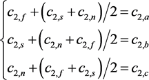(74)

Solving linear Equation (74) simultaneously gives

(75)

Note that the values of, , and are used to plot Figure 5 while the values of for triaxial shear tests listed in Table 1 are the final solution of equation (75).

4. Discussion

4.1. Anisotropic CSE Functional

In the anisotropic CSE functional, and instead of and are named and used albeit since the summation of invariant components or results in the corresponding invariant or

(76)

Moreover, the use of defined in (19) rather than in (13) captures anisotropic transverse deformations and avoids the unnecessary calculation of inverse right Cauchy-Green tensor.

In the anisotropic CSE functional (36), the first term, , represents the work done of normal stress and translational deformation. The second term, , describes the work done of shear stress and rotational deformation. The third term, , captures the work done of stress for finite deformations with different anisotropic degrees of ellipsoidal deformations.

With the fourth-order anisotropic elasticity tensor (38), the most general fourth-order elasticity tensor for isotropic hyperelastic materials can be recovered by the mappings of, , , …, and

(77)

Substituting the first and second order derivatives of invariants (6), (7), (8), and (9) into (77), simplifying, and rearranging produces

(78)

where the eight parameters are defined by

(79)

(80)

(81)

(82)

where the isotropic CSE functional is given by

(83)

The three constitutive constants, , and are generally used for modeling finite deformations of isotropic hyperelastic materials. The two constitutive constants, and, determine the isotropic elasticity tensor (78) with the eight parameters (79) through (82).

4.2. Comments on Different Experimental Tests

In uniaxial tension tests for SBTs, not only does the stress-stretch data in the tensile direction need to be captured but also at least one other orthogonal stretch must be measured for incompressible SBTs since needs to be evaluated for (19) in the CSE model, and transverse deformation effects on longitudinal deformations are indispensable in uniaxial tension tests. The transverse deformation effects in modeling SBTs has been elaborated on by Latorre, Romero, and Montáns (2016) [25] . With uniaxial tension measurements in the direction, for example, we also need to capture the corresponding transverse stretch or and use the incompressible condition to determine the other stretch or, respectively since and are generally not equivalent due to orthotropy. In constitutive modeling of the transverse uniaxial tension test of porcine liver tissues, the tensile stretch is and the shortenings of fibers and cross-fibers are and, respectively. Considering the anisotropic compression test results, the anisotropic contraction is simulated with and the constitutive constants have been obtained and listed in the PLT-T row in Table 1. If the isotropic contraction of were assumed, the constitutive constants would be and in which they are quite different from the PLT-T row of results in Table 1. Thus, it is essential to measure both the longitudinal and transverse stretches in uniaxial tension tests for incompressible SBTs.

In biaxial tension tests, it is very difficult to maintain both uniform force distribution and uniform normal deformations. In general, the stress-stretch curves in biaxial tension tests from cruciform specimens to square specimens are not accurate. For biaxial tension tests of square specimens, the stress as a function of stretch is generally overestimated. The overestimation, the correction factor, and the inverse finite element method regarding biaxial tension tests have been studied by Nolan and McGarry (2016) [26] . In the CSE models for biaxial tension tests, shear coupling effects do exist, making curve fittings harder. Without simplifications, at least four arguments, , , , and, have to be measured, causing material characterizations to be more complex.

In triaxial shear tests, according to different orthogonal fiber reinforcement orientations, shear deformations have been classified as longitudinal shear, perpendicular shear, and transverse shear by Destrade, Horgan, and Murphy (2015) [27] . The three orthogonal directions, fiber, sheet, and normal, for myocardial tissues generate six deformation modes: fiber-sheet mode, fibernormal mode, sheet-normal mode, sheet-fiber mode, normal-fiber mode, and normal-sheet mode. In the CSE model for triaxial shear tests, the longitudinal shear does not contribute any anisotropy, only the perpendicular shear elongates fiber reinforcements, and the perpendicular shear and transverse shear are coupled together. Without shear coupling effects, there would be three different experimental curves in the six deformation modes. The triaxial shear tests in six deformation modes for both porcine myocardial tissues by Dokos et al. (2002) [23] and human myocardial tissues by Sommer et al. (2015) [22] have produced more than three different curves, indicating shear coupling effects as well.

5. Conclusions

An anisotropic CSE functional, for isothermal processes, is postulated to be balanced with its stress work done, constructing a PDE. The anisotropic CSE PDE with respect to the three invariant components, , , and, is generally solved by Lie group methods. A three-term particular solution, which is essentially composed of ICGs, is particularly grouped by differential geometry to capture the three fundamental deformations. In a preferred direction i, the

term monitors translational deformations, the term captures

curvatures of rotational deformations, and the term describes curvatures of different powers of ellipsoidal deformations.

The anisotropic CSE constitutive models for uniaxial tension, biaxial tension, and triaxial shear tests have been derived. The constitutive constants have been solved by an iterative least square method for the uniaxial tension tests of rabbit abdominal skins and porcine liver tissues, the biaxial tension, and the triaxial shear tests of human ventricular myocardial tissues. With the newly defined second invariant component, the anisotropic CSE models capture the transverse effects in uniaxial tension deformations and the coupling effects between the perpendicular shear and transverse shear in triaxial shear deformations.

For anisotropic CSE models, the first constitutive constant, , can be treated as a dependent constant due to the ISF condition if necessary and the last three constitutive constants, , , and, are independent constants, defining the anisotropic elasticity tensor. For isotropic CSE models, the three constitutive constants, , , and, are needed for modeling finite deformations of isotropic hyperelastic materials. The two constitutive constants, and, are required for the isotropic elasticity tensor.

Acknowledgements

The author’s heartfelt thanks go to Jim S.J. Chen and Kenneth B. Margulies for their collaboration in earlier studies of rat hearts through ex-vivo tests of diastolic pressure as a function of balloon volume. He would also like to express his gratitude to Jianming and Jiesi Zhao for their discussion and assistance.

Conflicts of Interest

The authors declare no conflicts of interest.

References

[1]	Fung, Y.C. (1993) Biomechanics. Springer-Verlag, New York. https://doi.org/10.1007/978-1-4757-2257-4
[2]	Holzapfel, G.A. (2000) Nonlinear Solid Mechanics: A Continuum Approach for Engineering. John Wiley & Sons, Chichester.
[3]	Cowin, S.C. (2013) Continuum Mechanics of Anisotropic Materials. Springer, New York. https://doi.org/10.1007/978-1-4614-5025-2
[4]	Humphrey, J.D. (2003) Continuum Biomechanics of Soft Biological Tissues. Proceedings of the Royal Society of London A, 459, 3-46. https://doi.org/10.1098/rspa.2002.1060
[5]	Gasser, T.C., Ogden, R.W. and Holzapfel, G.A. (2006) Hyperelastic Modelling of Arterial Layers with Distributed Collagen Fibre Orientations. Journal of the Royal Society Interface, 3, 15-35. https://doi.org/10.1098/rsif.2005.0073
[6]	Holzapfel, G.A. and Ogden, R.W. (2010) Constitutive Modelling of Arteries. Proceedings of the Royal Society A, 466, 1551-1597. https://doi.org/10.1098/rspa.2010.0058
[7]	Chagnon, G., Rebouah, M. and Favier, D. (2015) Hyperelastic Energy Densities for Soft Biological Tissues: A Review. Journal of Elasticity, 120, 129-160. https://doi.org/10.1007/s10659-014-9508-z
[8]	Lanir, Y. (2017) Multi-Scale Structural Modeling of Soft Tissues Mechanics and Mechanobiology. Journal of Elasticity, 129, 7-48. https://doi.org/10.1007/s10659-016-9607-0
[9]	Spencer, A.J.M. (1971) Theory of Invariants. In: Eringen, A.C., Ed., Continuum Physics, Vol. 1, Academic Press, New York, 239-353. https://doi.org/10.1016/B978-0-12-240801-4.50008-X
[10]	Spencer, A.J.M. (1984) Continuum Theory for Strongly Anisotropic Solids. In: Spencer, A.J.M., Ed., Continuum Theory of the Mechanics of Fibre-Reinforced Composites, CISM Courses and Lectures, No. 282, International Centre for Mechanical Sciences, Springer-Verlag, Wien, 1-32.
[11]	Zheng, Q.-S. (1994) Theory of Representations for Tensor Functions—A Unified Invariant Approach to Constitutive Equations. Applied Mechanics Reviews, 47, 545-587. https://doi.org/10.1115/1.3111066
[12]	Schroder, J. and Neff, P. (2003) Invariant Formulation of Hyperelastic Transverse Isotropy Based on Polyconvex Free Energy Functions. International Journal of Solids and Structures, 40, 401-445. https://doi.org/10.1016/S0020-7683(02)00458-4
[13]	Itskov, M., Ehret, A.E. and Mavrilas, D. (2006) A Polyconvex Anisotropic Strain-Energy Function for Soft Collagenous Tissues. Biomechanics and Modeling in Mechanobiology, 5, 17-26. https://doi.org/10.1007/s10237-005-0006-x
[14]	Fung, Y.C. (1973) Biorheology of Soft Tissues. Biorheology, 10, 139-155. https://doi.org/10.3233/BIR-1973-10208
[15]	Holzapfel, G.A., Gasser, T.C. and Ogden, R.W. (2000) A New Framework for Arterial Wall Mechanics and a Comparative Study of Material Models. Journal of Elasticity, 61, 1-48. https://doi.org/10.1023/A:1010835316564
[16]	Zhao, F.Z. (2016) Continuum Constitutive Modeling for Isotropic Hyperelastic Materials. Advances in Pure Mathematics, 6, 571-582. https://doi.org/10.4236/apm.2016.69046
[17]	Zhao, F.Z. (2017) The Continuum Stored Energy for Constitutive Modeling Finite Deformations of Polymeric Materials. Advances in Pure Mathematics, 7, 597-613. https://doi.org/10.4236/apm.2017.710036
[18]	Itscov, M. (2000) On the Theory of Fourth-Order Tensors and Their Applications in Computational Mechanics. Computer Methods in Applied Mechanics and Engineering, 189, 419-438. https://doi.org/10.1016/S0045-7825(99)00472-7
[19]	Lanir, Y. and Fung, Y.C. (1974) Two-Dimensional Mechanical Properties of Rabbit Skin. II. Experimental Results. Journal of Biomechanics, 7, 171-182. https://doi.org/10.1016/0021-9290(74)90058-X
[20]	Tong, P. and Fung, Y.C. (1976) The Stress-Strain Relationship for the Skin. Journal of Biomechanics, 9, 649-657. https://doi.org/10.1016/0021-9290(76)90107-X
[21]	Chui, C., Kobayashi, E., Chen, X., Hisada, T. and Sakuma, I. (2007) Transversely Isotropic Properties of Porcine Liver Tissue: Experiments and Constitutive Modelling. Medical & Biological Engineering & Computing, 45, 99-106. https://doi.org/10.1007/s11517-006-0137-y
[22]	Sommer, G., Schriefl, A.J., Andra, M., Sacherer, M., Viertler, C., Wolinski, H. and Holzapfel, G.A. (2015) Biomechanical Properties and Microstructure of Human Ventricular Myocardium. Acta Biomaterialia, 24, 172-192. https://doi.org/10.1016/j.actbio.2015.06.031
[23]	Dokos, S., Smaill, B.H., Young, A.A. and LeGrice, I.J. (2002) Shear Properties of Passive Ventricular Myocardium. American Journal of Physiology-Heart and Circulatory Physiology, 283, H2650-H2659. https://doi.org/10.1152/ajpheart.00111.2002
[24]	Holzapfel, G.A. and Ogden, R.W. (2009) Constitutive Modelling of Passive Myocardium: A Structurally Based Framework for Material Characterization. Philosophical Transactions of the Royal Society A, 367, 3445-3475. https://doi.org/10.1098/rsta.2009.0091
[25]	Latorre, M., Romero, X. and Montáns, F.J. (2016) The Relevance of Transverse Deformation Effects in Modeling Soft Biological Tissues. International Journal of Solids and Structures, 99, 57-70. https://doi.org/10.1016/j.ijsolstr.2016.08.006
[26]	Nolan, D.R. and McGarry, J.P. (2016) On the Correct Interpretation of Measured Force and Calculation of Material Stress in Biaxial Tests. Journal of the Mechanical Behavior of Biomedical Materials, 53, 187-199. https://doi.org/10.1016/j.jmbbm.2015.08.019
[27]	Destrade, M., Horgan, C.O. and Murphy, J.G. (2015) Dominant Negative Poynting Effect in Simple Shearing of Soft Tissues. Journal of Engineering Mathematics, 95, 87-98. https://doi.org/10.1007/s10665-014-9706-5