The Water Problem and Its Solution in Gansu, China

Yuke Li¹, Luyi Wang², Hai Cheng³

¹School of International Studies, University of International Business and Economics, Beijing, China.
²School of Banking and Finance, University of International Business and Economics, Beijing, China.
³School of Information Technology and Management, University of International Business and Economics, Beijing, China.

DOI: 10.4236/am.2017.810110                

Abstract

Based on such severe situation, we need to work out a way that enables us to analyze the current and future ability of a region to provide clean water to meet the needs of its population, and to develop a reasonable strategy to optimize the utilization of water resources in this area. This paper has worked out a resolution model and input the data of China, the United States, Russia, Laos and Afghanistan to do national testing. Then, we use the policy from “diaper incident” to do policy testing. The calculation results of the model are in conformity with the reality. Therefore, the model is effective. At last this model is used to resolve Gansu’s water problem and provide effective advices for the local government.

Keywords

Water Scarcity, Water Supply Effect, China Resources Problems

1. Introduction

According to the UN water scarcity map, we find that the northern China is suffering from serious water scarcity. Some of the northern provinces in China even have achieved the degree of over-exploited, and Gansu province is included in these provinces. After conducting further investigation, we find that in Gansu province for many years, the average annual production capacity of surface water is 28.2 billion cubic meters, which accounts for 1% of the total surface water in China and ranks 29th out of 32 provinces (municipalities/ autonomous regions). The amount of water per acre reaches 378 cubic meters, which is about only a quarter of the national average and thus belongs to the serious water shortage areas. The per capita water capacity in Gansu is 1077 cubic meters, which is about one third of the national average, one-eighth of the world’s average and has been close to the international severe water shortage limits.

Therefore, we take Gansu province as a region where water is either heavily or moderately overloaded, which meet the requirements in task 2. We hope to find a way for Gansu province to alleviate water scarcity through this analysis.

2. Model Design

2.1. Model Building

2.1.1. A Brief Introduction of the Model

Since a detailed introduction has been stated in “2.1 Outline of the Solution”, thus we only make a simple explanation here as Figure 1.

As shown above, it is a dynamic model of water supply and demand, population, natural environment, GDP and time. Water supply and demand will have impact on population, and population will change the GDP and GDP per capita. GDP will directly influence the water supply and demand or indirectly influence the water supply and demand by changing the environment. Meanwhile, time is also able to influence the environment and thus change the water supply and demand.

2.1.2. The Operation Mechanism of the Model

a) Water Supply and Demand Model:

Water supply (s_k) is influenced by natural factors (a_w_k) and social facors ( $i_k$ ).

$s_k=a_0+a_1\times a\text{\_}{w}_k+a_2\times i_k+u_k$ (1)

1) Available water quantity model in the nature:

In the nature, available water quantity (a_w) is equal to the total water resources (z_w) minus the discharge [1] . In the formula, a₀, a₁ and a₂ are parameters that could be determined by the variance between supply (s_k) and natural factors (a_w_k) and social facors ( $i_k$ ), which is mainly indicated by the investment of water infrastructure, and u_k represents the residual error of the regression model. The model is:

Figure 1. Water supply relationship.

$a\text{\_}w=z\text{\_}w-10\times \text{discharge}$ (2)

Since the wastewater is discharged into the nature, it must produce pollution to other water resources. Here we assume that the polluted water is ten times of the sewage discharge.

2) Total water resource model in the nature:

Total water resource (z_w_k) in one region is in relation with the local precipitation, geology, topography and ecological environment. We assume that the influence of geology and topography to the total water resource is constant. The ability of a region to reserve water is mainly illustrated by forest coverage [2] . And the model is:

$z\text{\_}{w}_k=b_0+b_1\times {\text{precipitation}}_k+b_2\times {\text{forest\_area}}_k+u_k$ (3)

3) Precipitation model:

The atmospheric precipitation water can be calculated by surface vapor pressure. With recipitation model, we use surface temperature (T, unit: K) to calculate surface saturated vapor pressure (Ew, unit: hPa).

$\begin{array}{c}{\log }_{10}Ew=10．79574\times 1-\frac{273．16}{T}-5．02800\times {\log }_{10}\frac{T}{273．16}\\ +1．50475\times {10}^{-4}\times \left[1-{10}^{-8.2969\times \frac{T}{273．16}-1}\right]\\ +0．42873\times {10}^{-3}\times \left[{10}^{4．76955\times 1－\frac{273．16}{T}}-1\right]+0．78614\end{array}$ (4)

Then, we use the surface saturated vapor pressure and relative humidity (U, unit: %) to calculate surface vapor pressure.

$e=Ew\times U$ (5)

$U=\text{rpressure}/Ew$ (6)

The “rpressure” in the previous formula is the actual vapor pressure, so

$e=\text{rpressure}$ (7)

Because,

$\text{rpressure}=1.25a\left(1+t/273.15\right)$ (8)

“a” is absolute humidity in the previous formula. If a is constant and equals 10 (g/m³), then the precipitation is only related to the temperature. The model is:

${\text{precipitation}}_k=c_0+c_1\times {\text{rpressure}}_k+c_2\times {\text{rpressure}}_k^2+u_k$ (9)

4) Temperature model:

With greenhouse effect, the temperature t_k has the tendency of rising (n represents the year). It is because the growing influence of temperature to the precipitation [3] , we build the temperature model:

$t_k=d_0+d_1\times n+d_2\times n^2+d_3\times n^3+u_k$ (10)

5) Forest area model:

Since forest has a strong ability to reserve water, forest area $\left({\text{forest\_area}}_k\right)$ influences the local total natural water resources. After consulting materials, the forest area has a strong relation with GDP per capita (gdp_k) [4] . We build the forest area model:

${\text{forest\_area}}_k=e_0+e_1\times rgd{p}_k+e_2\times rgd{p}_k^2+e_3\times rgd{p}_k^3+u_k$ (11)

6) Investment in water infrastructure model:

Water infrastructure determines whether people can get more water to meet their needs. As is indicated in research, GDP per capita has dramatic impact on the investment in water infrastructure [5] . Imitating the lag variable models, we build this model to illustrate changes of investment in water infrastructure:

$i_k=f_0+f_1\times rgd{p}_k+u_k$ (12)

7) Waste water discharge model:

The amount of waste water discharge $\left({\text{rdischarge}}_k\right)$ has great influence on the amount of polluted water, which also changes the available water quantity. Referring to EKC research documents, we build this wastewater discharge model based on EKC relationship theory.

${\text{rdischarge}}_k=g_0+g_1\times rgd{p}_k+g_2\times rgd{p}_k^2+g_3\times rgd{p}_k^3+u_k$ (13)

8) Total waste water discharge model:

$\text{discharge}=p\times \text{rdischarge}$ (14)

b) Water demand model:

Water demand (d_k) is not only in relation with population, but also with economic development. We find the relation between water demand and GDP per capita in research documents, and build this model [6] :

$d_k=j_0+j_1\times rgd{p}_k+j_2\times rgd{p}_k^2+u_k$ (15)

c) GDP variation model:

After consulting related documents, we find the close relation between GDP and population (p_k). So we build the GDP variation model:

$gd{p}_k=m_0+m_1\times p_k+u_k$ (16)

d) Population model:

Because water is significant to human surviving, whether the water supply can meet the needs of water demand has considerable impact on the amount of population (p_k) [7] . Thus, we build this model:

$r_k=z_0+z_1\times s{d}_k+u_k$ (17)

$p_k=p_{k-1}\left(1+r_k\right)$ (18)

e) Finally, we use S/D to suggest the ability of a region to provide clean water to meet the needs of its population.

2.2. Model Testing

Application Analysis

We choose Shandong province as our research object to test whether the model is accurate and efficient. We get the data of Shandong province from 2005 to 2014 in China’s National Bureau of Statistics, and input these data into the model to conduct the test.

a) Water supply model:

$s_k=a_0+a_1\times a\text{\_}{w}_k+a_2\times i_k+u_k$ (1)

The result of regression analysis is Table 1.

The relationship between s_k and a_w is shown in Chart 1. The relationship between s_k and I is shown in Chart 2.

As Chart 1 and Chart 2 show, R-squared = 0.9515, which indicates this model explains the changes of s well. Since test value of P by F is close to 0, the model is statistically significant in general, and is moderate fine. Since the estimated value of coefficient of a_w is greater than coefficient of I, it suggests that water supply is more sensitive to the changes of a_w.

$s_k=198.742+0.0475029\times a\text{\_}{w}_k+0.0082295\times i_k$ (19)

Table 1.Linear regression 1.

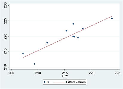
Chart 1. Available water quantity model (nature).

Chart 2. Available water quantity model (social investment).

Table 2.Linear regression 2.

The coefficient of a_w and I are both positive number, so s is in positive correlation with a_w and i.

1) Available water quantity model in the nature:

$a\text{\_}w=z\text{\_}w-10\times \text{discharge}$ (2)

2) Total water resource model in the nature:

$z\text{\_}{w}_k=b_0+b_1\times {\text{precipitation}}_k+b_2\times {\text{forest\_area}}_k+u_k$ (3)

The result of regression analysis is Table 2.

The relationship between z_w and precipitation is shown in Chart 3. The relationship between z_w and forest_area is shown in Chart 4.

The data represented in the above charts illustrate that R-squared = 0.8743, which indicates this model explains the changes of s well. Since test value of P by F is close to 0, the model is statistically significant in general, and is moderate fine. Since the estimated value of coefficient of precipitation is greater than coefficient of forest_area, it suggests that z_w is more sensitive to the changes of pre-

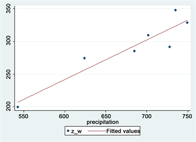
Chart 3. Precipitation and natural water supply.

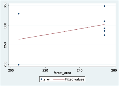
Chart 4. Forest area and natural water supply.

cipitation. Therefore, the model is:

$z\text{\_}{w}_k=-149.5273+0.5825711\times {\text{precipitation}}_k+0.1818078\times {\text{forest\_area}}_k$ (20)

The coefficient of forest_area and precipitation are both positive number, so z_w is in positive correlation with precipitation and forest_area.

3) Precipitation model:

${\text{precipitation}}_k=c_0+c_1\times {\text{rpressure}}_k+c_2\times {\text{rpressure}}_k^2+u_k$ (9)

The result of regression analysis is Table 3.

The relationship between Precipitation and rpressure as Chart 5.

R-squared = 0.3624, which indicates this model explains the changes of precipitation to some extent, but there are some errors. From the test result of F, the model is statistically significant in general, and is moderate fine. From the chart

Table 3.Linear regression 3.

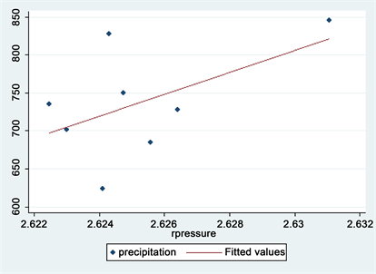
Chart 5. Precipitation model.

above, we could see that precipitation grows with rpressure in some condition. The model is:

${\text{precipitation}}_k=197e+07-1.50e+07\times {\text{rpressure}}_k+2858852\times {\text{rpressure}}_k^2$ (21)

4) Temperature model:

$t_k=d_0+d_1\times n+d_2\times n^2+d_3\times n^3+u_k$ (10)

The result of regression analysis is as Table 4.

The relationship between T and n is as Chart 6.

R-squared = 0.7638, which indicates this model explains the changes of temperature moderately, but there are some errors. Since test value of P by F is close to 0, the model is statistically significant in general, and is moderate fine. From the chart above, we could see that temperature grows with years in some condition. The model is:

$t_k=13.7568+0.4562897\times n-0.1736422\times n^2+0.0145319\times n^3$ (22)

Table 4.Linear regression 4.

Chart 6. Temperature model.

5) Forest area model

${\text{forest\_area}}_k=e_0+e_1\times rgd{p}_k+e_2\times rgd{p}_k^2+e_3\times rgd{p}_k^3+u_k$ (11)

The result of regression analysis is as Table 5.

The relationship between Forest_area and rgdp as Chart 7.

R-squared = 0.8099, which indicates this model explains the changes between forest_area and rgdp well, but there are some inevitable errors as well. From the test result of F, the model is statistically significant in general, and is moderate fine. From the chart above, we could see that forest area grows with GDP per capita in some condition. The model is:

$\begin{array}{c}{\text{forest\_area}}_k=265.2094-0.0827098\times rgd{p}_k+0.0000311\times rgd{p}_k^2\\ -2.95e-09\times rgd{p}_k^3\end{array}$ (23)

6) Investment in water infrastructure model:

$i_k=f_0+f_1\times rgd{p}_k+u_k$ (12)

Table 5.Linear regression 5.

Chart 7. Forest model.

Using the same regression analysis in water supply model, we can get the result of regression analysis is:

R-squared = 0.8099, which indicates this model explains the changes between investment and rgdp well, but there are some inevitable errors as well. From the test result of F, the model is statistically significant in general, and is moderate fine. From the chart above, we could see that investment grows with GDP per capita in some condition. The model is:

$i_k=-373.2892+0.431395\times rgd{p}_k$ (24)

7) Waste water discharge model:

${\text{rdischarge}}_k=g_0+g_1\times rgd{p}_k+g_2\times rgd{p}_k^2+g_3\times rgd{p}_k^3+u_k$ (13)

Using the same regression analysis in water supply model, we can get the result of regression analysis is:

R-squared = 0.9907, which indicates this model explains the changes between R discharge and rgdp well, but there are some inevitable errors as well. From the test result of F, the model is statistically significant in general, and is moderate fine. From the chart above, we could see that R discharge grows with GDP per capita in some condition. The model is:

$\begin{array}{c}{\text{rdischarge}}_k=15.8245+0.0069993\times rgd{p}_k+2.31e-07\times rgd{p}_k^2\\ -6.48e-11\times rgd{p}_k^3\end{array}$ (25)

Using the same regression analysis in water supply model, we can get these results:

b) Water demand model

$d_k=181.322+0.19625\times rgd{p}_k-2.31e-06\times rgd{p}_k^2$ (26)

c) GDP variation model:

$gd{p}_k=-677484+75.12275\times p_k$ (27)

d) Population model:

$r_k=-7876.886+7881.895\times s{d}_k$ (28)

All of these models are statistically significant in general, and the imitative effect is fine.

3. Gansu Province with Teh Model

3.1. Water Scarcity Analysis by Using Model

After analyzing the water supply and demand in Shandong, we use the data in the last 20 years provided by China’s National Bureau of Statistics and use the same method to build a model of water supply and demand in Gansu:

a) Water supply model:

$s_k=103.642+0.0572023\times a\text{\_}{w}_k+0.0162697\times i_k$ (29)

Available water quantity model in the nature:

$a\text{\_}w=z\text{\_}w-10\times \text{discharge}$ (30)

Total water resource model in the nature:

$z\text{\_}{w}_k=-173.4251+0.3355814\times {\text{precipitation}}_k+0.2315076\times {\text{forest\_area}}_k$ (31)

Precipitation model:

${\text{precipitation}}_k=54e+05-1.23e+04\times {\text{rpressure}}_k+2245751\times {\text{rpressure}}_k^2$ (32)

Temperature model:

$t_k=8.4534+0.3545827\times n-0.1369172\times n^2+0.0267482\times n^3$ (33)

Forest areas model:

$\begin{array}{c}{\text{forest\_area}}_k=434.1398-0.0593192\times rgd{p}_k+0.0001563\times rgd{p}_k^2\\ -4.26e-07\times rgd{p}_k^3\end{array}$ (34)

Investment in water infrastructure model:

$i_k=-174.3584+0.624367\times rgd{p}_k$ (35)

Waste water discharge model:

$\begin{array}{l}{\text{rdischarge}}_k=4.8565+0.0256297\times rgd{p}_k+1.91e-06\times rgd{p}_k^2\\ -3.58e-09\times rgd{p}_k^3\end{array}$ (36)

Total waste water discharge:

$\text{discharge}=p\times \text{rdischarge}$ (14)

b) Water demand model:

$d_k=104.624+0.26645\times rgd{p}_k-3.51e-07\times rgd{p}_k^2$ (37)

c) GDP variation model:

$gd{p}_k=m_0+m_1\times p_k+u_k$ (16)

d) Population model:

$r_k=-2893.527+3012.847\times s{d}_k$ (38)

$p_k=p_{k-1}\left(1+r_k\right)$ (18)

3.2. Water Situation in 15 Years

Time passes by 15 years from 2014, and we are in 2029. We use this model to forecast the water resources in Gansu, and here is the data as follows:

3.3. The Impact of This Situation on the Residents

According to the data, the value of S/D has changed into 0.92 < 1 in 2029, which suggests that the water supply is slightly insufficient. Though the total water resource and investment in water infrastructure has increased to some extent, both the GDP per capita and waste water discharge have increased which leads to a unobvious increase and even a loss in water supply. The increase in GDP per capita generates an obvious increase in water demand, and thus produces a scant water supply. Under this situation, on one hand the growth rate of population will fall, and reduce the water demand; on the other hand, government will increase the investment in water infrastructure, put a step forward on water conservation and utilization and increase water supply to make S/D ≥ 1 to meet the needs of water.

4. Intervention Plan

Design an Intervention Plan

Our intervention plan is made up of four parts: A, B, C, D.

Plan A: Alter the growing structure of crops

We should introduce a ban on large-scale reclamation, migration and high water-consuming plants in Hexi. Go a step further and reduce the planting area of intercropped wheat, corn and other common crops. Alleviate carrying capacities of resources by developing the cultivation of low water-consuming and drought-enduring plants. Expanding the planting area of wine grape and high- quality beer barley to achieve the win-win outcome of water saving and income increasing.

Plan B: Plant trees, thus expanding the forest areas

Expand the planting areas of forest and grass, increase the vegetation cover rate and strengthen the water-holding capacity of land.

Plan C: Increase financial expenditure on science and technology studies

Science and technology studies require the support from the financial policy. If science and technology studies receive more money, it will give a rise to the higher technological level of industrial production and irrigation, and thus reducing the industrial water consumption and agricultural water consumption.

Plan D: Increase financial expenditure on water infrastructure including water diversion and water conversion project

The Qinghai Lake is located closely to Gansu province, with which Gansu could conduct water conversion project that transforms the salt water in the lake into clean water. In addition, Gansu may construct water diversion project from nearby rivers. Both of the solutions will directly increase the water supply of Gansu. An increase of financial expenditure in water infrastructure will increase the amount of water diversion project, water harvesting project, water reserve project, water conversion project and pollution control project.

5. Conclusion

Historically, water scarcity has never been a trivial problem. Humans have always been seeking their ways when confronted with water scarcity. After consulting and analyzing the background information, we have summed up the previous attempts to exacerbate or alleviate the problem of water scarcity and come up with several causes for water scarcity. With the help of the model, China’s Government can promote such effective solutions for water scarcity to other provinces, which will bring some changes for the citizens living there.

Conflicts of Interest

The authors declare no conflicts of interest.

References

[1]	Deng, H.P. (2001) The Influence of Climate and Land Use Change on Hydrology and Water Resources Research. Advance in Earth Sciences, No. 6.
[2]	Li, Y., Zhang, J.D. and Luo, P. (2013) Atmospheric Precipitation Estimation Model Research. Meteorological and Environmental Sciences, No. 5.
[3]	Vapor Pressure Calculation Formula. http://wenku.baidu.com/link?url=I81MqdnJxQAc8WMfHQB7YvIzBsJqRIUq93bqY1NJNFeeRCRUAyH_b4nmye7uIghZ0b-gVsPZmvjoCl8DGhWAVKsvanSncTj3Ng-2MzetABC
[4]	Shi, C.N. and Wang, L.Q. (2006) An Econometric Analysis on Relations Between the Growth-Declining of Forest Resources and Economic Growth. Forestry Economic, No. 11.
[5]	Dong, M. and Lin, Y. (2007) Infrastructure Investment to GDP: Model, Relationships, and Conclusion. Journal of Inner Mongolia Finance and Economics College, No. 2.
[6]	Yin, J., Wu, Z.N. and Hu, C.H. (2007) Forecasting Model of Domestic Water Demand Related to GDP. Journal of Water Resources & Water Engineering, No. 4.
[7]	Liu, J.Q., Zheng, T.G. and Song, T. (2009) Environmental Pollution and Economic Growth in China: An Empirical Research Based on Linear and Nonlinear Methods. China Soft Science, No. 2.