Non-Linear Electrodynamics Gedanken Experiment for Modified Zero Point Energy and Planck’s “Constant”, h Bar, in the Beginning of Cosmological Expansion, So h(Today) = h(Initial). Also How to Link Gravity, Quantum Mechanics, and E and M through Initial Entropy Production in the Early Universe

Andrew Beckwith^*

College of Physics, Chongqing University, Chongqing, China.

DOI: 10.4236/jhepgc.2016.22016                

Abstract

We initially look at a nonsingular universe representation of entropy, based in part on what is brought up by Muller and Lousto. This is a gateway to bring up information and computational steps (as defined by Seth Lloyd) as to what will be available initially due to a modified Zero Point Energy formalism. The Zero Point Energy formalism is modified as due to Vissers’s setting of an angular plane number in early universe cosmology as k(maximum) ~ 1/(Planck length), with a specific initial density giving rise to initial information content which may permit fixing the initial Planck’s constant, h, which is pivotal to the setting of physical law. This will be in the spirit of Stoica’s removal of initial conditions of non-pathological initial starting points in Cosmology. What we want are necessary and sufficient conditions so h(today) = h(initial). We also in addition make a brief survey into 5th force arguments in gravity which also has a strict entropy interpretation. i.e., how to link gravity, quantum mechanics, and E and M through entropy production.

Keywords

Infinite Quantum Statistics, Gravitons

Received 5 November 2016; accepted 4 April 2016; published 7 April 2016

1. Introduction: Can h(Today) = h(Initial)? And What Is the Link of Quantum Mechanics, Classical Mechanics (Gravity) and Electromagnetics via Early Universe Entropy?

First of all, we wish to ascertain if there is a way to treat entropy in the universe, initially, by the usual black hole formulas. Our derivation takes advantage of work done by Muller, and Lousto [1] which have a different formulation of entropy cosmology, based upon a modified event horizon, which they call the Cosmological Event Horizon. i.e., it represents that the distance a photon emitted at time t can travel. Afterwards, we give an argument, as an extension of what is presented by Muller and Lousto [1] , which we claim ties in with Cai [2] , as to a bound to entropy, which is stated to be S (entropy) less than or equal to N, with N, in this case, a micro state numerical factor. Then, a connection as to Ng’s infinite quantum statistics [3] is raised. i.e., afterwards, we are then referencing C.S. Camara as a way to ascertain a non zero finite, but extremely small quantum bounce and then we use

the scaling, as given by Camara [4] , that a resulting density is scaled as by. The density of a given

cosmological equation of state of the universe, is proportional to a with a called the scale factor [5] , as of page 3 of [5] , which is a function of time which represents the relative expansion of the universe. Also, considering the elaboration given in [6] , we do a basic working definition of what a scale factor is.

One of the questions which have come up in discussion is what is meant by the term scale factor. In Cosmology, a as a scale factor is nearly zero at the start of the universe expansion, and equals 1 in the present era. In this case, a starts with a value just above zero, and obeys the cosmological Friedman equations. Scale factors are used as a convenient measuring convention in part in that the actual radii of the universe, and how it expands are controversial. By way of [5] [6] , we will have the following.

If time in the present era is set as ~13.7 billion years after the start of cosmological expansion of the universe, and say then by convention, seconds, i.e. a Planck time interval, then the following hold [5] [6]

, present era, (1)

Notice then that what we are referring to physically is that [5] [6]

(2)

So by definition,. In addition, we will set this scaling as a way to set minimum magnetic field values, commensurate to the modified Zero Point Energy density value, as given by Visser [7] , with paired off with [8] ’s rescaling of density, so then the magnetic fields as

given by [4] can in certain cases be then estimated. The reference to Planck length [8] and Planck mass [9] which is for the density calculation will permit, after accessing Walecka’s [10] result of comparison with a physical dimensional analysis derived time step (1), so by [10] we have

Time step (1) ~ 1/ square root of

(3)

This will be compared to another time step (2) based on [10] .

Time step (2) ~ 1/square root of

(4)

Further analysis will be assumed in the case where there is an equality between Equation (3) and Equation (4) so that by [4] we are giving further constraints upon magnetic fields and a cosmological “constant” [11] . The Cosmological constant for now is provisionally assumed to have today value, with

(5)

Doing so will then permit us to make further use of [12] and its relationship between a cosmological “constant” and an upper bound to the number of produced gravitons. The upper bound to the number of gravitons as given will be discussed as a way to ascertain if the cosmological constant, as given in Equation (5) evolves over time.

While here, will briefly allude to what the Cosmological constant did earlier and its role in present cosmological theory. As given by [13] the cosmological constant was put in place by Einstein in order to have a static universe. A static universe says that the universe no longer expands or contracts. That it is spatially not changing, in size over time. That there would be no situation where there would be a changing scale factor, i.e., to consider what this means look at the Equation (6) below.

The physical dynamics of how this constant works its way in, is in the following Einstein field equation, as given by page 180 of [13] leading to evolving scale factors, as given by the Friedman Equation of the form

(6)

When Equation (6) has no change in its size. Then one is then obtaining, with a nonzero curvature the physics saying that the universe has an invariant spatial domain we could render as, in the spirit of [14]

(7)

Realistically this Equation (7) would have the left hand side scale factor equal to 1, so then we would be having

(8)

This is in the case that we have non zero spatial curvature, i.e. if we have zero curvature, i.e. flat space, to have no energy evolution, the above becomes even simpler, i.e. the cosmological constant is negative. For a spatially invariant “repulsive” energy which would be the Left hand side of Equation (9) below

(9)

The left hand side of Equation (9) has a density in the case of zero curvature and invariant “repulsive” energy of

(10)

For the sake of understanding what G is, we could for the sake of argument, invent a cosmology for which, with to be defined as below as in the fifth force arguments, i.e. as the value of a gravitational constant at the far distance between two masses, call them. We will elaborate upon that identification of at the end of the introduction, but we will in general identify G namely as the strength of gravity, and ignore situations for which G may vary over time, as given in [15] . For now if G is the strength of gravity, and invariant, we will further state what this to expect about the cosmological constant.

The supposition that the cosmological constant was put in place was initially a way to have repulsive “anti- gravity” so as to have the static universe, as what was considered the case in 1917. And duplicated above, the dynamic universe also is tied into suppositions that the cosmological constant may be the driving force behind re acceleration of the universe, as given in [16] , namely if the cosmological constant, as given by the last term in Equation (6) is assumed to be vacuum energy, then it can lead to a situation for which we can have expansion accelerating via the scale factor by the rule of

(11)

The other situation which will comment upon is a situation for which the “cosmological constant” may in some sense vary over time, i.e., an easy example will be given below by using reference [12] , where the number of gravitons, as a measure of entropy, will be connected with the “cosmological constant”.

Note that by Peebles, N, as a particle number count as in the radiation era, is usually conflated with entropy [17] . Which is also confirming [2] [3] . Further elaborations are given in [12] . Isolating N (the number of gravitons) and if this is commensurate with entropy due to [2] [3] will allow us to use Seth Lloyd supposition of [18] as to the number of permitted operations in quantum physics may be permitted. This final step will allow us to go to the final supposition, as to what number of operations/information may be needed to set a value of h (Planck’s constant) in the beginning of the universe with invariant over time. Note that what Seth Lloyd is doing is the result of making a relationship between computational bits, of information producing cosmic computer operations, in explicit relationships. What we will do, is to use the Ng identification [3] of entropy, S ~ N, a count of gravitons, initially produced, with this number then equal 3/4^th in power magnitude to the number of computational cosmic computer steps taken by a cosmic “computer”. i.e. what we will see later is that the gravitons produced up to the present day will be about 10^90, equal to the 3/4^th power of 10^120, where the value of 10^120 is the number of operations necessary to produce the equivalence of initial Planck constant, h(initial) with today’s value of Planck’s constant h(today) [19] , with

(12)

Note that h(today) was the proportionality constant between the minimal increment of energy of a hypothetical electrically charged oscillator in a cavity that contained black body radiation, and the frequency of its associated electromagnetic wave. In 1905 the value of minimal energy increment of a hypothetical oscillator, was associated by Einstein with a “quantum” of the energy of the electromagnetic wave itself. The light quantum eventually was called the photon. This is what [19] is about, and our paper is to indicate conditions permitting

in Equation (12). It is closely tied into what is calculated as of Equation (18) below, a one meter or so initial radii, for.

In addition we will make the following identification of entropy with the following fifth force argument. The two arguments about entropy will be re enforcing each other, and we will talk about what the two entropies portend to, in our conclusion.

So as this is the introduction, before we go to develop the first part of our introduction, we will briefly access 5^th force arguments here. This fifth force argument and what it portends to, will be compared to the main developed argument given above, in terms of its effect upon entropy, in the conclusion.

We start off with a description of both the Fifth force hypothesis of Fishbach [20] - [22] as well as what Unnishkan brought up in Rencontres De Moriond [23] [24] with one of the predictions dove tailing closely with use of gravitons as produced by early universe phase transition behaviour, leading to how QM relates to a semi classical approximation for E and M and other physical processes. For the Fifth force used, we use the following from Fishbach [20] namely what is admittedly an oversimplified model, as

(13)

The generalized charges, Q, as brought up are defined, briefly in Equation (13) in the next few lines, whereas the term is a range of a presumed 5^th force, with, as given by [20] is ~1000 to 2000 meters in length, whereas if we look at the masses are frequently of values of 1 GeV/c^2, i.e. ten to the ninth electron volts, i.e. obviously if we were identifying gravitons, that they would, if they had any mass be massively accelerated almost to the speed of light, and that due to the rest mass of a graviton usually identified as to be about 10^−62 grams, or about 5.5 times 10^30 electrovolts/C^2. As given by [25] . In addition the term as given in Equation (13) (7) as which is the value of the interaction between the two masses as the spatial distance between them goes to infinity.

This second term in the potential, in Equation (13) is going to have, here fifth force charges we will outline as having the magnitude as defined by the following dimensional analysis of

(14)

We have that Unnishkan shared in Rencontres Du Moriond [23] [24] which is an extension of what he did in [24] i.e. looking at, if are currents in electricity and magnetism, and are the “Newtonian” “gravity” equivalent expressions, with mass 1 and mass 2, and velocities of the two particles in question so that the following, up to a point holds. If, and

are the masses of Equation (14) with the following relation given to the author by Unnishkan when he gave [23] [24] as a way to link gravity with electromagnetic forces. This note, given to the author has some similarities to [26] as given by Ciufolini and Wheeler.

(15)

This is where Unnishkan would have to be coherent with the prior formalism identification of charges and of mass, a setting of Equation (16) below to help us make sense of a genuine connection between Electro magnetics and gravity. The Left hand side of Equation (16) is E and M. and up to a point similar to Equation (9) whereas the right hand side of Equation (16) is gravity, similar to the right hand side of Equation (15). Here the term is a potential function term which will play a role in a linkage of E and M and Gravity. See [27]

(16)

We argue that the linkage of Equation (16) of magnetism with mechanics, and by default gravity, is similar in part to what Ciufolini and Wheeler wrote up in [26] as their work with the initial value problem in Einstein Geometrodynamics, pp 271-314, and this connection will be further explored in follow ups in our research. Keep in mind what [27] is referring to which has some analogies to our work is on page 280 of their book in a read starting under the title “Hilbert Choice of Action Principle Supplies Natural Fixer of Phase for Getrodynamics” with page 287 then getting very close to our work, under the Heading “An interpretation: The Analogy with Electrodynamics”. In particular the feed into the page 288 Equation (5.2.29) in [27] is in spirit very close to what we are doing here, a similarity which will be explored in future publications.

The above relationship as in Equation (15) and Equation (16) with its focus upon interexchange relations between gravity and magnetism is in a word focused upon looking at, if A, the nominal vector potential used to define the magnetic field as in the Maxwell equation, the relationship we will be using at the beginning of the expansion of the universe, is a variation of the quantized Hall effect, i.e., from Barrett [21] , the current I about a loop with regards to electronic energy U, of a loop with the A electromagnetic vector potential going through the loop is given by, if L is a unit spatial length, and we approximate the beginning of the universe as having some of the same characteristics as a quantized Hall effect, then, if n is a particle count of some sort, then by [27]

(17)

We will be taking the right hand side of the A field, in the above, and approximate Equation (17) as given by

(18)

Then, we have an approximation for writing a modification of [27] we will give as

(19)

Equation (19) needs to be interpolated, up to a point. I.e. in this case, we will conflate the n, here as a “graviton” count, initially, i.e. the number of early universe gravitons, then assume that is a net acceleration term which will be linked to the beginning of inflation, i.e. that we look then at Ng’s “infinite” quantum statistics [3] [28] , with entropy given as, initially a count of gravitons, with a generalized count. Then, if,

and we refer to the n of Equation (17) to Equation (19) as being the same as, keeping in mind some pitfalls of entropy in space-time considerations as given in [3] [28]

(20)

We will elaborate upon this treatment of entropy in our derivations, and compare this behaviour of entropy in the first part of our introduction, which is for coming up with entropy as far as a way to confirm if or not we can preserve Planck’s constant, from cycle to cycle of presumed universe creation to its collapse (if that happens) plus its recreation (recreation of the universe after collapse). The significance of linking E and M, Classical Mechanics, Quantum processes, and entropy via 5^th forces will be in showing the unity of entropy production of classical (gravity) predictions, QM, and electromagnetics in terms of how we could maintain the constancy of physical law, due to evolution equations of physics which would have invariant physical constants, i.e. no change during cosmological evolution.

2. Calculations as to Entropy, and What It Says about Bouncing, versus Non-Singular Universes?

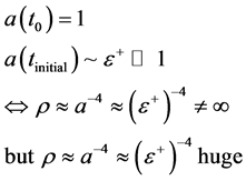
The term non-singular universe is short hand for an initial starting point as to the expansion of the universe which is not at a singular point of space-time. Reference [4] begins with this supposition, as well as does [24] [29] i.e. the quantum bounce idea of Loop quantum gravity. Keep in mind we are also using the Non-Linear Electrodynamics non-zero singularity which is also a nonzero bounce for the start of the universe [30] [31] . Having said that, such effects do seem to tie in also with work the author has done in [32] which is in its own way a partial confirmation of [29] as a starting point. We will use this while assuming in our calculations does not go to zero. In this paper, this radii, is similar to what is done in black hole physics, as is noted by [1] , and gets to the heart of the entropy calculation. That we are modeling the acquisition of initial nonzero entropy in the universe with a one to one equivalence with black hole physics is what motivates the rest of this paper. In doing so, we will urge more advanced readers of this document to access [33] to get an idea of how tricky this initial condition stuff in early universe cosmology actually is.

For the record, the usual interpretation of in terms of black hole physics, is in terms of what is called an event horizon. An event horizon is a boundary in space-time beyond which events cannot affect an outside observer, i.e. in black hole physics, once a person passes through this radial distance from a black hole, it supposedly is such that the observer cannot escape the pull of the black hole gravity gradient.

So, we will assume a linkage between black hole physics event horizons, as defined, and early universe cosmology in the manner brought up by [1] .

We begin first by putting the results of [1] here and subsequently modifying them. To begin with, we look at what was given as to entropy, and this was actually asked me as to a review of a similar article several weeks ago. By [1] , a(grid) ~ Planck’s length. Note that this is not the same thing as the scale factor! As given by [1]

(21)

The specifics of what were done with, is what will be discussed in this section, and Equation (1) has its counterpart as given by, if R is the radius of a sphere inside of which harmonic oscillation occurs, and is in this case is of a different value, i.e. generalized Harmonic Oscillator based lattice spacing [1] .

(22)

The main import of Equation (20) is that it defacto leads to a “non-dimensional” representation of entropy, but before we do that, it is useful to review what is said about. As defined in [1] , is called the maximal co-ordinate distance a photon can travel in space-time in a given time, t.

FWIW, we will provisionally in the regime of z (red shift) > 1100 set for inflation from a Planck time interval up to 10^-20 seconds, when the expansion radii of the universe was about a meter, i.e.

(23)

What we will do in later parts of this paper, to get an approximation as to what the actual value of is, and to use this to comment upon the development of entropy.

a. Relevance of Equation (23) to the concept of dimensionless entropy

Cai, in [2] has an abbreviated version of entropy as part of a generalized information measurement protocol which we will render as having T.F.A.E.

(24)

We will assume that, and then connect the entropy of Equation (22) with Ng’s entropy [3] with the result that

(25)

While assuming Equation (24) we will through [3] be examining the consequences of infinite quantum statistics for which, if the “Horizon” value as defined above is made roughly commensurate with say graviton wavelength, with also consideration of

(26)

The entropy so mentioned, above, is commensurate with the following identification, namely how to link a measure of distance with scale factor. We will as a starting point use the following identification, namely start with the radiation dependence of [4]

(27)

Our starting point for the rest of the article will lie in making sense of the following inputs into the scale factor as the last part of Equation (26) grouping of mathematical relations, namely we will look at time defined via

[10] . of time And the following for defining the density, via its scaled relationship to, with the minimum value of, as given by Camara [4] as, using a frequency, an initial E

and M field given at the start of creation itself, and of course a cosmological “constant” parameter, with the following linked to a minimum scale factor, i.e. if we look at Camara [4] , keeping in mind that c is the speed of light and that G is invariant.

The author is for now avoiding a time varying G, as it is creating Partial Differential equations the author has no idea of how to solve, for the time being, so we assume that G is invariant and use the Equation (28) result at this time [34]

i.e.

(28)

Then we use, by [4]

(29)

The linkage to graviton mass, and heavy gravitons will build upon this structure so built up via [25] , and will comprise the capstone as to what to look for in GW research. A topic which the author is involved with, i.e. consequences of working with the following implied graviton mass will be brought up, namely by [33] and assuming a present rest mass of the graviton as given by [35]

(30)

This above formula will de evolve, from a larger value, to having the mass of a graviton approximately as given about 10^−62 grams in the present era [25] . Also, if the above graviton mass is accepted, we will be considering the value of N defined within the event horizon, with [36]

(31)

A specified value of will also be ascertained, in this document. We set it equal to 1, and then calculated the other values from there. From the above, we will specify a variance graviton mass, a minimum time, according to the above, and work out full consequences, with suggestions for finding exact values of the above parameters.

3. Filling in the Parameters, What It Says about Initial Cosmological Conditions?

First, now the treatment of entropy due to early universe Gravitons. In the beginning of this analysis, we start with Ali and Das’s cosmology from Quantum potential article [35] , where a derived cosmological “constant is given by, if meters squared, and meters squared, so that

(32)

Equation (11) should be compared to an expression given by Padmanabhan [37] , if the, and, and

(33)

Then the entropy at the end of the electro weak era is, assuming this is commensurate with graviton production, with the value of the Horizon radius at the upper end of Equation (32) above, namely about 1 meter

(34)

Given this, we can now consider what would be the magnetic field, initially, and the other parameters as given in the end of the last section. Doing so, if so, we can have frequency as high as

(35)

Using inflation, this would be redshifted at a minimum of 11 orders of magnitude, down to about 10^10 Hz today, at the highest end. The nature of the E and B fields, also as fill in would have to be commensurate with what was given in [36] .

Still though, as a rule of thumb, we would have that the MINIMUM value of the magnetic field, in question would have to be [4] , i.e. for high frequencies, the minimum value of the magnetic field would actually be very low!

(36)

4. 1^st Part of Conclusions: Why We Have a Non-Zero Initial Entropy, and How to Unify the EM, QM, CM, Gravitational and Other Variants of Entropy?

Why we pursued this datum of an initial nonzero entropy? In a word, to preserve the fidelity of physical law from cosmological cycle to cycle, i.e. the bits we calculated with, came from Seth Lloyd [18] , and also from Giovannini [38] , with the upper end to graviton frequencies calculated as [18]

(37)

Lloyd, sets, in [18]

(38)

The first part of Equation (37) in terms of “bits” is approximately similar to Equation (38), and more tellingly,

(39)

The upper part of Equation (38) overlaps, a bit with Equation (37) whereas Equation (36) is only a few orders of magnitude higher than the formal numerical count for the number of operations, # of Equation (39), i.e. the number of bits, given in Equation (39) is similar to the graviton entropy count given in Equation (32), However, most tellingly, the initial non zero graviton count, given when the universe is 1 meter in diameter, or so, is initiated by negative pressure, which we recount, below.

We state, first of all, that with we use Lloyd [18] , and also Corda, et al. [39]

(40)

The upshot is that the entropy, at the close of the inflationary era, would be dominated by graviton production as of about the electroweak era, and this would have consequences as far as information, as can be seen by the approximation given by Seth Lloyd [18] on page 14 of the article [18] as to the number of operations # being roughly about

(41)

In the electro-weak era, we would be having Equation (42) as giving a number of ‘computational steps’ many times larger (10 orders of magnitude) than the entropy of the electro-weak,

(42)

In addition, making use of the above calculations, if we do so, we obtained that the minimum time step would be of the order of Planck time, i.e. of about 10^−44 seconds, which is very small, but not zero, whereas, again, assuming a 1 meter radii, which we obtain at the end of inflation, with a time step the, at the end of inflation of 10^−20 seconds. This is significant, when the universe had a radii of 1 meter, is about when we would expect r to be about 1 meter to then get us a value of Equation (42) in upper bound, i.e., setting r about 1 meter would allow us to have to have the upper bound value of Equation (41) being that of Equation (36).

This set of number of operations would be about when we would expect Planck’s constant to be set, with the values as given in [18] .

Finally, we assert that the following are equivalent, namely in the pre Planckian era, just before the onset of the big bang

(43)

The is of Planck Length [32] , i.e. this is for space time with values just before the big bang. The E field so derived is roughly of the same magnitude of the B field as given in Equation (30). The presence of the function is the same as what is in Equation (19), and so then with a preservation of bits of information and ini-

tial entropy, i.e., bits, it would be possible to have.

We include below the derivation of Equation (43) which is for showing the following equivalences given in Electromagnetism, Quantum Mechanics, Classical Mechanics, and Gravity, through foundational Entropy at the Pre-Planckian level.

Equation (43) is a direct result of the following derivation, namely see the below, with Q, here, a fifth force quantity.

Entropy, Its Spatial Configuration near a Singularity and How We Use This Definition to Work in Effects of Non-Linear Electrodynamics

The usual treatment of entropy, if there is the equivalent of an event horizon is, that (Padmanabhan) [39] with to be set at the end of the article, with suggestions for future work. And L order of magnitude proportional to, i.e., we will suggest a formal relationship between L and. Here we leave this as to be a determined parameter

(44)

If so, then we have that from first principles, (and here we also will set formally at the end of the paper, with suggested updates as far as an investigation)

(45)

Then Equation (7) is re written in terms of [23] [24] adopted formulation as given by

(46)

The following parameters will be identified, i.e. what is, what L is, and what is. These values

will be set toward the end of the manuscript, with the consequences of the choices made discussed in this document as suggested new areas of inquiry. However, Equation (46) will be linkable to re writing Equation (16) as

(47)

If is ALMOST time independent, as we will assert in the end of our paper, Equation (47) will then lead to a primordial value of the magnitude of the A vector field as

(48)

We should, here, keep in mind that that abbreviation of H.O.T. means higher order terms. Sometimes they are extremely important, and other times that happens not to be the case.

If so, then the E field up to a point will be

(49)

To reconstruct we have that we will use

(50)

Then

(51)

If so, then in Equation (49) becomes

(52)

The density, then is read as

(53)

The current we will work with, is also then linkable to, by order of magnitude similar to Equation (53) of

(54)

Then we get an effective magnetic field, based upon the NLED approximation given by Corda et al. [39] of

(55)

Then we can also talk about an effective charge of the form, given by applying Gauss’s law to Equation (53)

(56)

This charge, Q, so presented, will be part of the effective 5^th force [23] [24] , as to linking E and M and gravity, of Equation (13) which we will relate to our further derivational work done in this paper. Furthermore, the criti-

cal value of which will be made explicit in this paper, as well as L, and as well as

(57)

This will lead to an evaluation of as

(58)

The value of (speed of light), and by Padmabhan [38] , , so then most likely then the

following are equivalent and imply each other as given in the grouping called Equation (43). This all is in keeping with [40] . Keep in mind that in reviewing Equation (57) especially, that we should keep our final results in fidelity with [41] and to delineate what is correct in [41] and what we are building upon, as a possible augmentation to Einstein’s great insights.

In [42] , there is a reference as to “stochastic background radiation of a primordial nature or resulting from the superposition of a large number of individually unresolvable sources”. What we are doing with Equation (57) and Equation (58) is to find conditions for identifying stochastic radiation of primordial origin and to avoid the multiple sources. To a large degree, this is the basic motivation of our fifth force inquiry. In addition, it requires getting the input from Equation (55) as to a primordial magnetic field correct, and that to avoid the problem of Bicep 2, in which dust messes up the gravitational waves. To aid in that, the frequency associated with the magnetic field, in Equation (55) as well as measurements in graviton counts, as may occur in a correct reading of Equation (44), as a graviton count per unit area of space, have to be done in adherence to [43] , as well as the inputs of coupling between electromagnetic fields from the primordial processes referred to in this document. [44] also is important in this investigation as to investigating our claim that the interferometric tests for the fidelity of our model with measurements as to [44] will be aided by correct evaluation of Equation (44), Equation (55) and of course Equation (57) and Equation (58), i.e. the existence of explicit 5^th force arguments will aid greatly in determining the choice of either general relativity or Scalar-Tensor theories of gravity as the origin of early universe primordial gravitational wave, and/or electromagnetic phenomenon. We assert that since [1] conflates early universe conditions with stars, that an early universe condition equivalent to the redshift of reference [45] will appear, and that it will be important in terms of making certain our signals, are primordial and avoid the trap is mentioned in [42] of stochastic background due to multiple signals. Same as in [46] . A correct reading of redshift, and its NLED contributions, for gravitational physics are a datum which should be investigated carefully so as to keep the problems of [42] vintage, especially avoiding contamination of the early universe signals with the BICEP 2 multiple sources problem. Equation (44), Equation (55), Equation (57), and Equation (58) are relevant to a counter part to the Born-Infeld NLED section of reference [45] . In particular, note that [45] has a long Section 3.2 which delineates constraints upon the magnetic field for what is called in [45] an effective metric. We can use a derived magnetic field we have in our document in lieu of the “Equation (32) and Equation (33) and Equation (34) and Equation (35)” of [45] to come up with a similar analysis for our early universe conditions. When done, we hope that this work will also enable a deeper inquiry as to what Corda raised in reference [44] as a procedure to investigate the fidelity our work with one of the models of gravity prevalent in the cosmology community as well as its fidelity or divergence with the outstanding work done by Einstein in reference [41] . While using fully the methodology given in [46] to full effect.

Acknowledgements

This work is supported in part by National Nature Science Foundation of China grant No. 11375279.

Conflicts of Interest

The authors declare no conflicts of interest.

References

[1]	Mueller, R. and Lousto, C.O. (1995) Entanglement Entropy in Curved Space-Time with Event Horizons. Physical Review D, 52, 4512-4517. http://dx.doi.org/10.1103/PhysRevD.52.4512
[2]	Cai, R.-C. (2005) Some Remarks on Constant Curvature Spaces. In: Liu, K. and Yau, S.-T., Eds., Superstring Theory, Higher Education Press, Beijing, 234-250.
[3]	Jack Ng, Y. (2008) Space-Time Foam: From Entropy and Holography to Infinite Statistics and Nonlocality. Entropy, 10, 441-461.
[4]	Camara, C.S., de Garcia Maia, M.R., Carvalho, J.C. and Lima, J.A.S. (2004) Nonsingular FRW Cosmology and Non Linear Dynamics. Arxivastro-ph/0402311 Version 1.
[5]	Weinberg, S. (2008) Cosmology. Oxford University Press, Oxford, 3.
[6]	Schutz, B. (2003) Gravity from the Ground up: An Introductory Guide to Gravity and General Relativity. Cambridge University Press, Cambridge.
[7]	Visser, M. (1996) Lorentzian Wormholes, from Einstein to Hawkings. AIP Press, Springer Verlag, Baltimore, Maryland.
[8]	http://physics.nist.gov/cgi-bin/cuu/Value?plkl
[9]	http://physics.nist.gov/cgi-bin/cuu/Value?plkm
[10]	Walecka, J.D. (2008) Introduction to Modern Physics, Theoretical Foundations. World Press Scientific Co, Pte. Ltd., Singapore, 596224.
[11]	Carmeli, M. and Kuzmenko, T. Value of the Cosmological Constant: Theory versus Experiment. https://cds.cern.ch/record/485959/files/0102033.pdf
[12]	Haranas, I. and Gkigkitzis, I. (2014) The Mass of Graviton and Its Relation to the Number of Information According to the Holographic Principle. International Scholarly Research Notices, 2014, Article ID: 718251. http://www.hindawi.com/journals/isrn/2014/718251/
[13]	Grupen, C. (2005) Astroparticle Physics. Springer-Verlag, Berlin.
[14]	https://cosmology.carnegiescience.edu/timeline/1917
[15]	Dungan, R. and Prosper, H.B. Varying-G Cosmology with Type Ia Supernovae. Submitted to the American Journal of Physics. http://arxiv.org/abs/0909.5416
[16]	Dyson, L., Klebana, M. and Susskind, L. (2002) Disturbing Implications of a Cosmological Constant. Journal of Cosmology and Astroparticle Physics, 2002, 0210:011. http://arxiv.org/pdf/hep-th/0208013v3.pdf
[17]	Peebles, P.J.E. (1993) Principles of Physical Cosmology. Princeton University Press, Princeton.
[18]	Lloyd, S. (2002) Computational Capacity of the Universe. Physical Review Letters, 88, Article ID: 237901. http://arxiv.org/abs/quant-ph/0110141 http://dx.doi.org/10.1103/physrevlett.88.237901
[19]	Taylor, B.N. and Mohr, P.J. (2015) 2014 CODATA Recommended Values. They are generally recognized worldwide for use in all fields of science and technology. The values became available on 25 June 2015 and replaced the 2010 CODATA set. They are based on all of the data available through 31 December 2014. http://physics.nist.gov
[20]	Fishbach, E. and Talmadge, C. (1988) The Fifth Force: An Introduction to Current Research. In: Fackler, O. and Tran Thanh Van, J., Eds., Fifth Force Neutrino Physics, VIII, Moriond Workshop, Editions Frontiers, Gif-sur-Yvette, 369-382.
[21]	Fishbach, E. and Talmadge, C. (1999) The Search for Non Newtonian Gravity. Springer-Verlag, Heidelberg.
[22]	Fishbach, E. (2015) Rencontres De Moriond, 2015, Gravitational Physics Section. http://moriond.in2p3.fr/J15/transparencies/4_wednesday/2_afternoon/5_Fischbach.pdf
[23]	Unnikrishnan, C.S. (2015) Dynamics, Relativity and the Equivalence Principle in the “Once-Given” Universe. http://moriond.in2p3.fr/J15/transparencies/3_tuesday/2_afternoon/7_Unnikrishnan.ppt
[24]	Unnikrishnan, C.S. (2014) True Dynamical Tests of the Weak Equivalence Principle for Matter and Anti-Matter. International Journal of Modern Physics: Conference Series, 30, Article ID: 1460267. http://www.worldscientific.com/doi/pdf/10.1142/S2010194514602671 http://dx.doi.org/10.1142/s2010194514602671
[25]	Goldhaber, A. and Nieto, M. (1974) Mass of the Graviton. Physical Review D, 9, 1119-1121. http://dx.doi.org/10.1103/PhysRevD.9.1119
[26]	Ciufolini, I. and Wheeler, J.A. (1995) Gravitation and Inertia. Princeton Series in Physics, Princeton University Press, Princeton.
[27]	Barret, T.W. (2008) Topological Foundations of Electromagnetism. World Scientific Series in Contemporary Chemical Physics, Vol. 26, World Scientific, Singapore.
[28]	Beckwith, A. (2011) Is There a Generalized Way to Represent Entropy? Prespacetime Journal, 2, 737-742.
[29]	Haggard, H.M. and Rovelli, C. (2015) Black, Hole Fireworks: Quantum Gravity Effects outside the Horizon Spark Black to White Hole Tunneling. Physical Review D, 92, Article ID: 104020. http://arxiv.org/abs/1407.0989 http://dx.doi.org/10.1103/PhysRevD.92.104020
[30]	Corda, C. and Mosquera Cuesta, H.J. (2011) Inflation from R Squared Gravity: A New Approach Using Non Linear Electrodynamics. Astroparticle Physics, 34, 587-590. http://dx.doi.org/10.1016/j.astropartphys.2010.12.002
[31]	De Lorenci, V.A., Klippert, R., Novello, M. and Salim, J.M. (2002) Nonlinear Electrodynamics and FRW Cosmology. Physical Review D, 65, Article ID: 063501. http://dx.doi.org/10.1103/physrevd.65.063501
[32]	Beckwith, A. (2015) Gedankenexperiment for Refining the Unruh Metric Tensor Uncertainty Principle via Schwartz- shield Geometry and Planckian Space-Time with Initial Nonzero Entropy and Applying the Riemannian-Penrose Inequality and Initial Kinetic Energy for a Lower Bound to Graviton Mass (Massive Gravity). Ukrainian Journal of Physics. http://vixra.org/abs/1509.0173
[33]	Galloway, G., Miao, P. and Schoen, R. (2015) Initial Data and the Einstein Constraints. In: Ashtekar, A., Berger, B., Isenberg, J. and MacCallum, M., Eds., General Relativity and Gravitation: A Centennial Perspective, Cambridge University Press, Cambridge, 412-448.
[34]	Haranas, I. and Gkigkitzis, I. (2014) The Mass of Graviton and Its Relation to the Number of Information According to the Holographic Principle. International Scholarly Research Notices, 2014, Article ID: 718251. http://www.hindawi.com/journals/isrn/2014/718251/
[35]	Padmanabhan, T. Accessed 22 November 2015. http://ned.ipac.caltech.edu/level5/Sept02/Padmanabhan/Pad1_2.html
[36]	Wen, H., Li, F.Y., Fang, Z.Y. and Beckwith, A. (2014) Impulsive Cylindrical Gravitational Wave: One Possible Radiative form Emitted from Cosmic Strings and Corresponding Electromagnetic Response. The European Physical Journal C, 74, 2998. http://arxiv.org/abs/1403.7277 http://dx.doi.org/10.1140/epjc/s10052-014-2998-9
[37]	Ali, A.F. and Das, S. (2015) Cosmology from Quantum Potential. Physics Letters B, 741, 276-279. http://dx.doi.org/10.1016/j.physletb.2014.12.057
[38]	Giovannini, M. (2008) A Primer on the Physics of the Cosmic Microwave Background. World Scientific, Singapore. http://dx.doi.org/10.1142/6730
[39]	Corda, C. and Cuesta, H. (2010) Removing Black Hole Singularities with Non Linear Electrodynamics. Modern Physics A, 25, 2423-2429.
[40]	Padmanabhan, T. (2010) Gravitation, Foundations and Frontiers. Cambridge University Press, New York. http://dx.doi.org/10.1017/CBO9780511807787
[41]	Einstein, A. (1917) Cosmological Considerations in the General Theory of Relativity. Sitzungsber. Preuss. Akad. Wiss, Berlin (Math.Phys.), 1917, 142-152.
[42]	Van Den Broeck, C. (2015) Gravitational Wave Searches with Advanced LIGO and Advanced Virgo. In: Augé, E., Dumarchez, J., Van, J.T.T., Eds., Proceedings of the 50th Rencontres de Moriond, “Gravitation: 100 years after GR”, ARISF, Paris. http://arxiv.org/abs/1505.04621
[43]	Das, S., Mukherjee, S. and Souradeep, T. (2015) Revised Cosmological Parameters after BICEP 2 and BOSS. Journal of Cosmology and Astroparticle Physics, 2015, 016. http://arxiv.org/abs/1406.0857 http://dx.doi.org/10.1088/1475-7516/2015/02/016
[44]	Corda, C. (2009) Interferometric Detection of Gravitational Waves: The Definitive Test for General Relativity. International Journal of Modern Physics D, 18, 2275-2282. http://arxiv.org/abs/0905.2502 http://dx.doi.org/10.1142/s0218271809015904
[45]	Mosquera Cuesta, H.J. and Salim, J.M. (2004) Nonlinear Electrodynamics and the Gravitational Redshift of Highly Magnetised Neutron Stars. Monthly Notices of the Royal Astronomical Society, 354, L55-L59. http://arxiv.org/abs/astro-ph/0403045 http://dx.doi.org/10.1111/j.1365-2966.2004.08375.x
[46]	Mosquera Cuesta, H.J. and Salim, J.M. (2004) Nonlinear Electrodynamics and the Surface Redshift of Pulsars. The Astrophysical Journal, 608, 925. http://iopscience.iop.org/article/10.1086/378686 http://dx.doi.org/10.1086/378686