Performance Indicators for Sun-Tracking Systems: A Case Study in Spain ()
1. Introduction
According to [1] , when radiation traverses a medium, each molecule or particle attenuates energy. Attenuation is a function of the type and the number of molecules in the path of a solar ray. It results evidently that the number of molecules or particles a solar ray strikes before reaching the ground is related to the distance traversed by the ray. Thus, beam radiation is more energetic than diffuse or reflected radiation, and that fact boosts the photovoltaic phenomena (the solar radiation can provide the enough energy to overcome the energy gap in the semiconductor material).
A sun-tracker is a machine that is designed as a mounting for photovoltaic panels so that they track the sun in such a way that the incident angle of solar radiation with the panels is as less as possible, thereby increasing energetic production with respect to fixed systems. Many types of solar trackers exist, which vary in terms of cost and complexity [2] .
We can classify the sun-tracker mechanisms according to:
1) Their control system;
2) The movement they perform.
According to the control system, sun-trackers are usually divided into active controlled sun-trackers and passive controlled sun-trackers [2] . The active controlled sun-trackers use motors and mechanical systems to transmit them the correct movements for sun-tracking. These movements are commanded by a controller which can be based on photosensitive cells (which can detect the direction of the maximum light flux) or chronological systems [3] [4] . These systems are precise. But, on the other hand, they are complex and with high rates of maintenance. Due to the motors consuming energy, continuous movements are commonly prevented. It is preferred to use step movements to save energy. Their associated costs are related to their precision accuracy. The passive controlled sun-trackers can be based on memory shape alloys or, more often, in the use of two cylinders and a liquefied gas with a low ebullition point. These kinds of systems are quite imprecise and they are not appropriate for certain applications (as for example concentration photovoltaic systems) [5] [6] .
On the other hand, the different models of trackers can be classified according to the movements they perform, in the following way:
1) Single-axis polar-mount trackers. This kind of trackers are devices with a fixed N-S axis set at an appropriate tilt angle which acts as the rotation axis of the photovoltaic panels (see Figure 1(a)).
2) Horizontal-axis trackers. They have a horizontal axis allowing seasonal tracking of the sun (see Figure 1(b)).
3) Vertical-axis or azimuth solar trackers. In this case, the panel array rotates about a fixed vertical axis for daily tracking (see Figure 1(c)).
4) Dual-axis solar trackers. These devices offer better performance by enabling daily (E-W) and seasonal (N-S) solar tracking. They can be based on different configurations: polar-mount, rotating platform or parallel kinematics (see Figure 1(d)).
There is no ideal tracker device for all possible installation cases. It is needed to take into account the advantages and disadvantages for each tracking policy [7] -[10] .
Of particular interest of this study, according to [11] more than 1/3 of the installations in Spain have sun tracking: 24% have 2-axis tracking and 13% have 1-axis tracking. The rest are fixed systems.
2. Material and Methods
To analyze the real performance of sun trackers in Spain, we have collected data along 4 years (2008-2011) about energy production of 3 real PV plants located in Spain. Data sets have been adequately analyzed and filtered in order to prevent outliers or deviations from the real behavior. It should be noticed that the first year data correspond with the first year life of the installation, which is not really representative due to several malfunctions and problems it occurred until normal operation. Thus, data from first year have been pondered adequately.
All the analyzed plants are located very close and all have near the same configuration options (PV arrays configurations, wiring distribution, inverters…) to compare the results of the different tracking systems. PV panels are not exactly the same but their electrical characteristics and Performance Ratios in Standard Test Conditions are quite similar (see Table 1).
Moreover, we have taken into account the estimated global radiation for each PV plant thanks to a solar radiation database: Photovoltaic Geographical Information System (PVGIS) [12] , which is one of the most commonly used nowadays. PVGIS incorporates a solar radiation database and gives climatological data of Europe. This system

Table1 PV plants parameters.
makes it possible to calculate long-term average values and daily profiles of the irradiation on PV modules [7] .
PVGIS needs data on solar radiation in order to make estimates of the performance of PV systems and to do the other calculations possible in the web application. There exist a number of different sources of solar radiation data, but none of them are perfect, so it is important to understand the strengths and weaknesses of each data source. In the new version of PVGIS (autumn 2010), it is included a choice of solar radiation databases for some regions. The two main sources of data on solar radiation on the earth’s surface are [7] :
1) Ground measurements.
2) Calculations based on satellite data.
In this case we preferred the New PVGIS database based on satellite measurements because it includes data from the same time period (2008-2011) we analyze [13] .
It is important to notice that the PVGIS system does not allow the user to simulate a horizontal-axis tracker directly. For that case we simulated the installation as a fixed one with different tilting angles from 15 deg. to 55 deg. with 5 deg. step, such as the real installation currently works.
3. Results
In this section we are going to compare the average behavior of the different PV plants described before.
3.1. Production Analysis
Table 2 shows the estimated global radiation obtained from PVGIS on a horizontal surface (Hm) and on the generator plane (Gm) recorded from each PV plant. The Gm value is always higher than the Hm value because the sun-tracking advantage affects it. Figures 2(a)-(c) shows the differences between both datasets and Figure 2(d) shows the standard deviation values between the 3 locations.
It can be noticed that standard deviations are quite small in comparison with the average value for the horizontal surface dataset (less than 3% in all cases). On the other hand, standard deviation for the Gm value is quite higher due to it implies the sun-tracking improvement. According to these data the dual-axis tracking plant can gather 692 kWh/(m2∙year)more than a fixed one; and the horizontal-axis one can gather about 242 kWh/(m2∙year) in advance.
Table 2. Estimated global radiation on an horizontal surface (Hm) and on the generator plane (Gm).
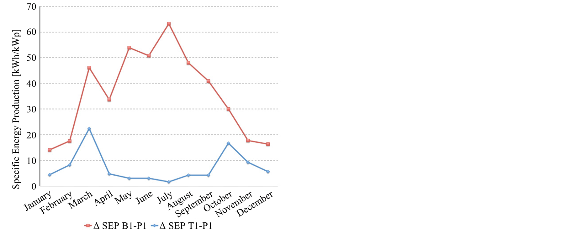
Energy measurements from each installation are shown in Table3 Original measurements cannot be compared due to the different power sizes of each plant. Thus, we have calculated the Specific Energy Production (SEP) and it shows that the most productive system is the dual axis one. Figure 3(a) represents the differences between the SEP values for each month on each plant in comparison with the fixed system (P1). For the one-axis tracking facility, these differences are greater in spring and autumn, but for the dual-axis system differences are greater in summer.
As PV plants have not the same power sizes and they are not located exactly at the same place (although it has been seen that the standard deviation for the incident global radiation on an horizontal surface is less than 3% at any case) we must take care about the parameter we compare in order to decide which system is working the best. That parameter, or set of parameters, must be independent from power size and location (incident global solar radiation). The performance ratio (PR) described in Equation (1) reaches both conditions. It compares the measured energy production per photosensitive square meter (which is proportional to the installed peak power) and the global radiation on a horizontal surface per square meter (Hm) that gathers each PV plant. We do not use the global irradiation on the generator plane (Gm) due to it just will give us the electrical performance of the PV panels and it does not depend on the sun tracking.
 (1)
(1)
Em is the measured energy production [kWh], n is the number of PV panels in the installation [units], SPV is
Table 3 . Measured energy production (Em) and Specific Energy Production (SEP) for each analyzed PV plant.
 (a)
(a)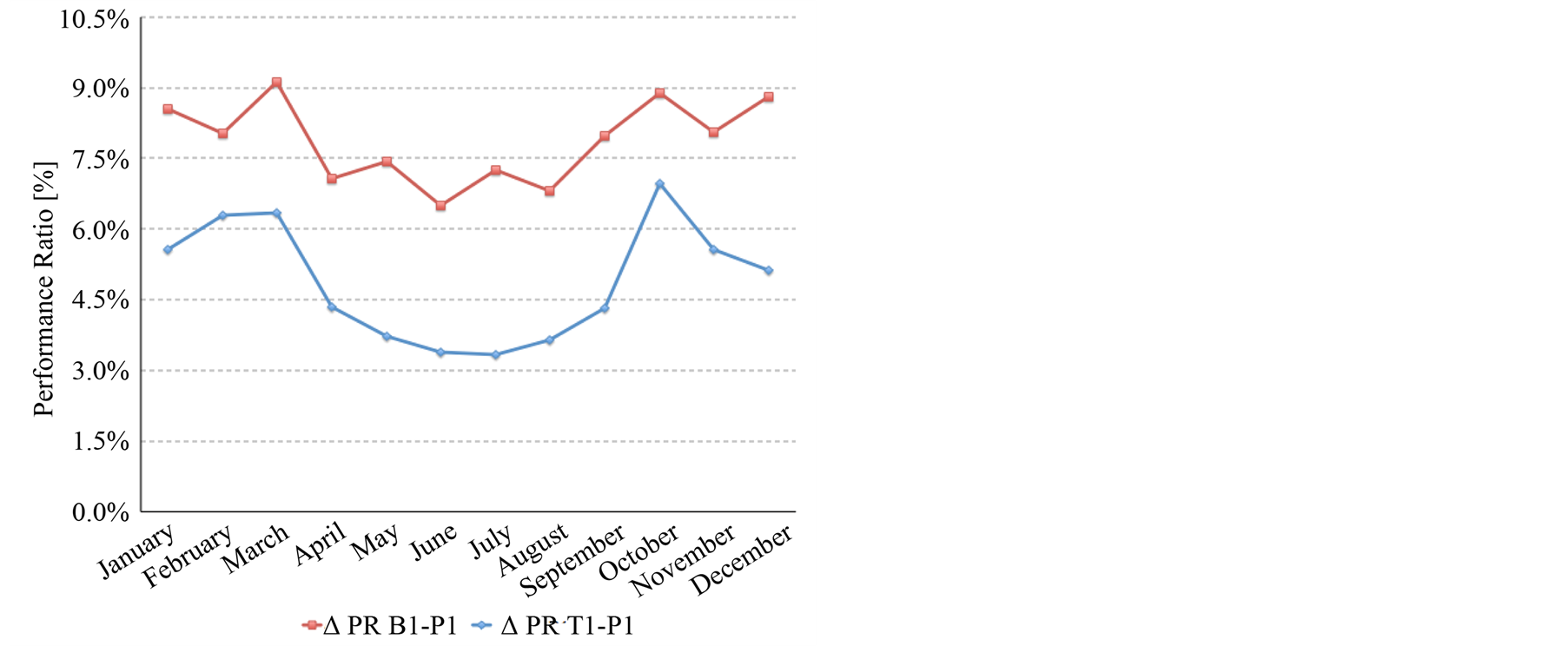 (b)
(b)
Figure 3. Differences between the SEP values (a) and PR (b) of plants T1 and B1 respect to plant P1.
the photosensitive region of each PV module [m2] and Hm is the global radiation on the PV panel [kWh/m2]. Thus, the performance ratio is then obtained unitless.
We can see in Table 4 the PR value for each month of the year corresponding to each PV plant. Differences respects to the fixed system (P1) are shown in Figure 4(b).
3.2. Surface Performance Ratio
Table 5 analyzes the effect of the surface needed for each sun-tracker system. The area occupied for each system has been determined by applying the procedures described in [9] [14] [15] .
Some authors use a parameter called Ground Cover Ratio (GCR) [8] [16] , which is defined as the ratio of the
Table 4 . Performance Ratio (PR) for each PV plant along an average year.
Table 5. Surface performance ratio analysis.
 (a)
(a)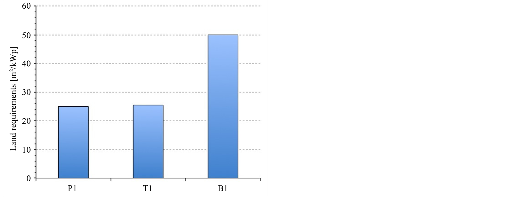 (b)
(b)
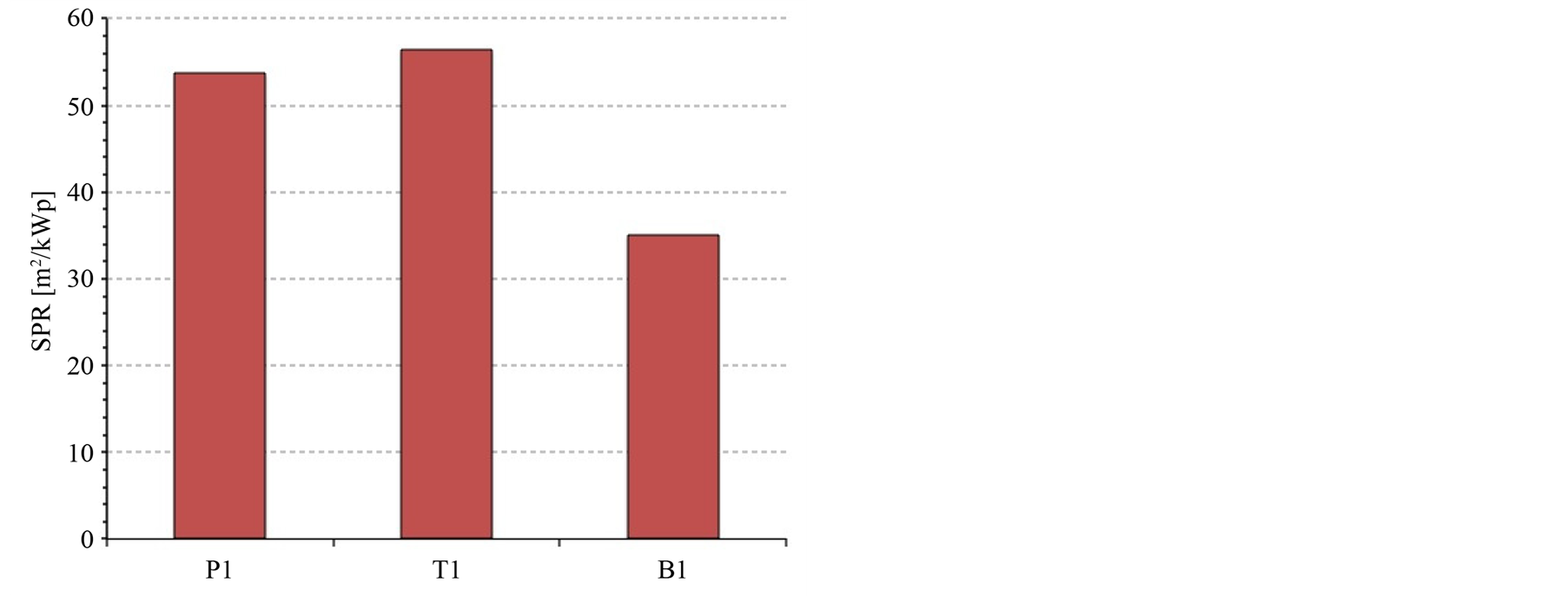
Figure 4. (a) Land requirements comparison; (b) Surface Performance Ratio for each system.
PV array area to total ground area for the system. The higher value the GCR has, the better surface exploitation is done [17] .
However, we use an equivalent but more representative parameter called Surface Performance Ratio (SPR). This has been defined as the product of the Specific Energy Production ( ) and the peak power installed per land square meter (P/S), as it is shown in the following Equation (2).
 (2)
(2)
The SPR takes into account not only the production improvement of the tracking system, but the larger area it needs for the installation. It should be noticed that the SPR value is independent of the power size of the installation.
Figure 4(a) shows that the horizontal-axis tracking system needs similar land requirements than the fixed mounting device. On the other hand, the dual-axis sun-tracker needs near the double land per kWp. Therefore the SPR for the last kind of tracking has near 40% less value than a fixed system. The horizontal-axis tracker has 4.24% better value (see Figure 4(b)).
3.3. Financial Analysis
We finally have carried out a financial study including the most commonly used financial parameters for each plant-Payback Time (PBT), Net Present Value (NPV) and Internal Rate of Return (IRR).
For the PBT analysis it has been taken into account the real costs of the investment (I) [€], the retribution of the produced energy (c) [€/kWh] and maintenance and replacement costs (m) [€/year]. This value has been calculated with Equation (3),
 , (3)
, (3)
where p is the yearly energy production of the installation in kWh/year. Results are shown in Table6
The investment value in this case involves the final cost of the whole installation, including PV panels, inverters, transformers, wiring, mounting structures or tracking devices, labor costs and taxes. The first line in Table 6 represents the results for the investment costs per peak power. It also can be seen that the highest costs are associated with the dual-axis system. On the other hand, the fixed mounting installation and the horizontal-axis one have approximately the same costs about 6000 €/kWp. This is due to the installation configuration is near the same and the fixed structure and the seasonal tracker are very similar. The horizontal-axis system is slightly cheaper than the fixed mounting due to the size costs distribution. The costs of investment of the dual-axis tracker installation achieve 8000 €/kWp. Data agree with the average costs of this sort of installations. Energy retribution has been calculated according to [18] and the electrical energy market along the considered time period.
The third line in Table 6 compares the PBT value for the different PV plants including the analyzed costs and the energy production. Results show that a fixed mounting configuration needs about 12 years to return the initial investment, a horizontal-axis one only needs 10 years, but a dual-axis installation requires almost 13 years.
The NPV has been calculated for each plant according to Equation (4),
 (4)
(4)
where I is the initial investment [€], R is the cash flow per considered period [€], i is the desired interest rate for the investment (opportunity cost) [no units] and n is the number of periods [years]. Equation (3) can be used only if the cash flows (R) are the same for each period. The desired interest rate has been fixed to 3.5% which was the average interest value for fixed-term deposits in 2007-2008 [19] . The study has considered 25 years as the investment period because it is the widely considered useful life for this sort of plants [6] .
The IRR is the value for I when the NPV comes to zero. As Equation (4) is not an explicit one the IRR has been calculated by numerical techniques. Both results for NPV and IRR for each plant are shown in Table7
Results from the financial analysis show that the most profitable plant is T1, which has horizontal-axis tracking. The worst investment is the dual-axis installation B1, with a remarkable low IRR value. It should be noticed that in line 6 in Table 7 the Net Present Value (NPV) has been normalized dividing by the power size of each plant (Specific NPV) in order to obtain a more descriptive parameter. It presents its best value for the T1 plant.
4. Conclusions
Table 8 collects all the parameters obtained in order to compare the 3 studied installations. SEP is higher in spring and autumn seasons for the horizontal-axis tracking plant, but higher in summer for the dual-axis tracking installation. This conducts us to think that, for the studied latitude, azimuth-tracking is more effective in summer and slope-tracking is more relevant in spring and autumn.
PR values in tracking plants are always higher than in the fixed one. As expected, PR value from the dual-axis plant is always higher in the whole year. Furthermore, it can be observed that major improvements correspond to the spring and autumn seasons for both tracking plants. Dual-axis tracking improves on average almost 3% more than the horizontal-axis tracking and almost 7.5% more than the fixed system.
Analyzing the land requirements through the SPR parameter we find out the best result for the horizontal-axis system. Furthermore, dual-axis tracking achieves worse results even than the fixed installation. Thus, although in the case study dual-axis tracking collects more than 30% energy than a fixed mounting system, the excessive land requirements—due to the shadows it projects—makes this system quite less effective. This is the reason why we consider dual-axis tracking in the studied conditions only profitable in concentrated photovoltaic systems (CPVs) or isolated ones.
Finally, according to the carried out financial analysis, we can conclude clearly that, for the case study, the most worthy investment is the horizontal-axis installation. This plant returns the initial investment almost 12% earlier than the fixed one, and about 20% earlier the dual-axis system. This conclusion is also supported by the NPV and the IRR analysis. The achieved IRR value around 8.5% is quite competitive in the investment market. However, we should remember that this analysis has been carried out under the hypothesis that the energy retribution remains constant along the 25 years of expected life for the PV plants. Otherwise, results can be different.
Table 8. Parameters for sun-tracking performance analysis.
In the case study, the dual-axis tracking facility shows the best performance from the strictly energetic point of view, but in real practice, when we take into account the land restrictions and the economical profitability, the horizontal-axis tracking plant beats clearly the other systems.
Acknowledgements
This work was partially supported by the Spanish Government (grant ENE2011-27511) and the Department of Culture and Education of the Regional Government of Castilla y León (grant BU358A12-2).