1. Introduction
The urban climate has been studied by several researchers who seek to understand the urban limit layer (UBL) and changes caused by different land uses. This is a complex layer due to the energy flow and the constant friction causing turbulence and transport of energy and mass, in the first 2 km of the atmospheric layer. The city structure substantially modifies the transport of energy and momentum in UBL changing the local climate, requiring an in-depth study on this process.
Planning policies using urban design tools should be applied by city managers to minimize the negative impacts of urban climate, especially in tropical climate cities.
There is a requirement for a more comprehensive and multidisciplinary approach, including different groups of researchers, such as geographers, architects, meteorologists and sociologists, in an attempt to find an urban model that promotes energy saving and mitigates climate change that may be occurring. The integration between urban and vegetation is a key issue in most cities where speculation causes intense urban spaces occupation, giving priority to concrete and asphalt at the expenses of green areas. The use of vegetation is a common tool in environmental projects to reduce energy consumption, suppressing the formation of heat and providing thermal comfort.
Gómez et al. (2003) conducted a bioclimatic study in Valencia, Spain, using thermal comfort indexes ID (thermal discomfort index), WBGT index (globe temperature) and PE (cooling) to analyze the influence of vegetation on human comfort and found a significant correlation between these elements.
Lahme and Bruse (2003) conducted a study on microclimate and air quality in the region of Essen, Germany, using measurements on site and Envi-met model, comparing the results. The model reproduced data collected on site with some accuracy, using equipment installed at these locations.
Ahmed (2003) conducted a study on the tropical urban environment in Dhaka, Bangladesh and found that the ratio and the internal and external environment must be studied. The author measured temperature and humidity in July and August in different areas of the city, namely: areas of low density of buildings and areas of high density of residential and industrial construction. According to the author, providing a microclimate comfort is linked to urban design (geometry, orientation of buildings, building materials, plant mass and water bodies) and energy saving.
Gomes and Amorin (2003) conducted a study of thermal comfort in urban space in Presidente Prudente—SP, BRAZIL. The authors used the effective temperature index developed by Thom (1959), which defines comfort zones, with dry bulb and wet bulb temperature data. Areas with larger arborization were thermally comfortable compared to those without arborization.
Researchers have found that not only building materials, with their high rates of heat storage, but also the height and structure of buildings, which form the so-called urban canyons can influence the temperature values and comfort in the city. This study focuses on the thermal comfort related to urban architecture, in an attempt to obtain the best building structure in favor of local users. Four cases of ground cover were used, at the central block.
This area consists of buildings and vegetation on the ground. Another area with grass covering, which replaced the buildings in the block by medium-density grass, a grassy area known as “grass/tree”, with the addition of 58 broad foliar trees of 15 m in height and one last area called “park” also added of grass and trees up to 15 m in height over the entire area.
Study Area
The study area of Ourinhos is located in southeastern Brazil and has subtropical climate with dry winter and rainy summer.
This city is located near the Tropic of Capricorn, presenting in this area many rivers, and Paranapanema River is the main river. The Turvo and Pardo Rivers are tributaries of the Paranapanema Rivers and these two rivers, despite being smaller, present large volumes of water. In addition to these rivers, Ourinhos shelters more than one hundred of springs, so this is a propitious region to produce relatively high humidity, especially in the warmer months.
During the months from May to July, there are more frontal systems from the southern end of South America, causing temperature decline and low humidity. Blockages are also important atmospheric climate dynamics, causing intense Indian summer, generating long periods of drought. This contributes to atmospheric stability, which provides temperature inversions, trapping the particles from sugar cane burning, and aerosols from soil preparation by farmers. On the other hand, from September to March, there is an increase in solar radiation in the Southern Hemisphere, and an increase in relative humidity. This causes many days with thermal discomfort. It is noteworthy that both in the winter and summer, the population has problems with thermal discomfort due to excessive cold or heat, because the built environments are not prepared to meet the needs of people in relation to the issue of thermal comfort.
In months from May to July, there is a predominance of frontal systems from the southern end of South America, leading to declining temperature and low humidity.
From September to March, with increasing solar radiation in the Southern Hemisphere, there is an increase in relative humidity, rising the temperature and causing many days of thermal discomfort. It is noteworthy that both in the winter and summer, the population has problems with thermal discomfort due to excessive cold or heat, because the built environments are not prepared to meet the needs of people in relation to the issue of thermal comfort.
The city of Ourinhos presents mean temperature of 23.1˚C, in which February and March are the hottest months and June and July the coldest. The average annual rainfall is 1405.3 mm and the wettest months are November, December and January (summer) and the driest are June, July and August (winter), as shown in Table1
Ourinhos (Figure 1) has urban area of 40 km2, rural area of 256 km2, covering an area of 296 km2. The city population of 109,228 inhabitants—IBGE 2005, and population density of 367.45 inhabitants per km2 according to IBGE—present urbanization level of 96.3%.

Table 1. Temperature and precipitation—Ourinhos, SP.
Data: http://www.Ciiagro.Sp.Gov.br (CIIAGRO, 2010) (Period: 05/01/2000 to 02/08/2010).
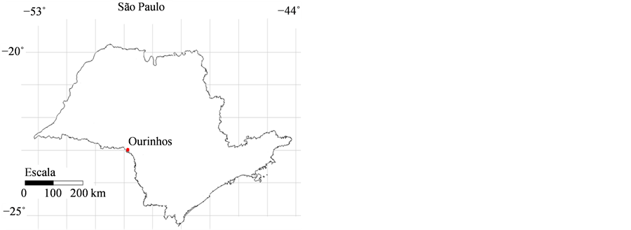
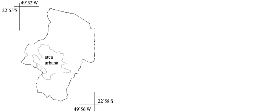
Figure 1. Maps of São Paulo state and county of Ourinhos.
It also presents an area of woods and forests of 398 hectares and an area of natural pastures of 1703 hectares (IBGE 2006). The chosen site covers an area of 3 × 3 blocks in the city downtown (Figure 2), which is located in the middle block, where the Water Service and Sanitation Provider (SAE) building can be found. In this place an automatic weather station was installed.
This is essentially a business area, but with the presence of some houses of one floor and ceramic roof tiles. There is also a building of 45 m of height in concrete slab roofing and some buildings with metal roofing.
2. Materials and Methods
The Envi-met version 3.0/3.1, three-dimensional micro-climate designed model was used to simulate the surface-plant-atmosphere interaction in the urban environment, with a resolution between 0.5 and 10 m. This model was developed by Bruse and Fleer (1998) and Bruse (2004). The edition of the floor plan on the urban area was made as a model of input data. The floor plan was designed in a scenario in three dimensions (3D), where buildings and trees/vegetation were placed on different surfaces.
Four simulations were made on the same day with different structures for the study area, changing the ground covering in an attempt to reproduce scenarios that might result in better thermal comfort indices. First, we used an actual area (Figure 3). This area consists of real buildings and existing vegetation on the site, then an area called “grass” where buildings were replaced in the middle square by grass of intermediate density (Figure 4), then a grassy area known as “grass/tree” with an addition of 58 broad leaved trees up to 15 m in height (Figure 5) and a final area called “Park” also grassed and with the addition of trees covering the entire area and up to 15 m in height (Figure 6). For each simulation, we chose a point within the grid for a more detailed study of the meteorological variables.
A file containing information on temperature, wind speed, relative humidity at 6 a.m. was inserted. These data were obtained from an automatic station installed at the SAE building, located in the central block of the study area.
It was inserted a file containing information on temperature, wind speed, relative humidity, at 6 a.m. obtained by an automatic weather station installed in the building of SAE, on middle block area of study. These values were: T = 293.0 K (18.0˚C), Vv = 0.8 m/s and RH = 80.0%. Air temperature, specific humidity, and sensible heat fluxes, wind speed and PMV (predicted mean vote) and PPD (percentage of dissatisfied people) indexes were compared in the areas of the four proposed structures.

Figure 2. Google Earth image of the study area with the SAE (Water Service and Sanitation Provider) building at the center block.
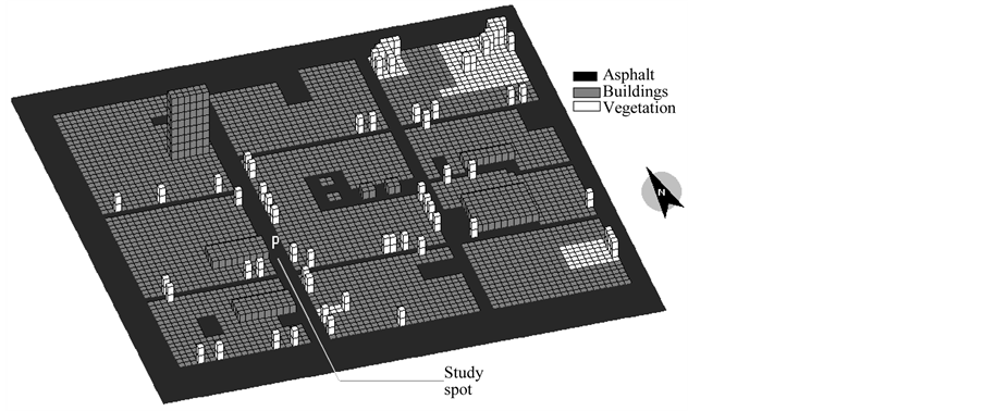
Figure 3. Study area with the location of a study spot on the asphalt to the actual area.
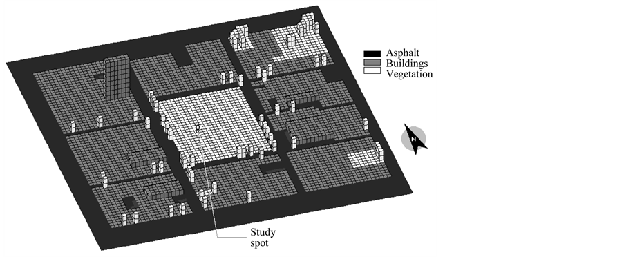
Figure 4. Location of the study area for simulation two (II) with the introduction of grass cover on the middle block and location of a study on the grass.
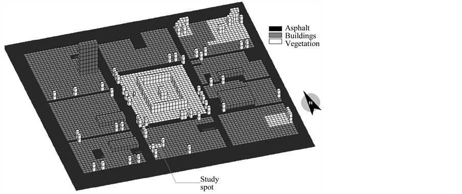
Figure 5. Location of the study area for simulation three (III), introducing grass and trees coverage on the middle block and location of a study on the grass.
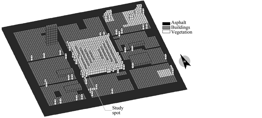
Figure 6. Location of the study area for simulation four (IV) with the introduction of trees on the middle block and location of the study spot.
The PMV is a bio-meteorological index, based on the model of Fanger (1972), which refers to the energy balance of people’s bodies exposed to certain climates. Originally developed for interiors, it was adapted for external environment, Jendritzky (1993).
Typically, the PMV range is defined from −3 (very cold) to +3 (very hot), where zero is the neutral (comfort). PMV as a function of the local climate could also reach values above 3 or below −3. In the PMV index, the ENVI-met model provides the PPD index value, which indicates the percentage of people who were dissatisfied with the climatic conditions. To evaluate the thermal comfort, various types of indices and models have been adopted. In this work, the PMV/PPD was used, which is used in ISO international standard (International standards 7730/1994).
ISO 7730 aims to present a method for predicting the thermal sensation and degree of discomfort for people exposed to moderate thermal environments and specify acceptable environmental conditions for comfort.
A compound is considered comfortable when the PPD heat index value does not exceed the value of 10.0%, according to the aforementioned ISO 7730/94. According to ISO 7730, the recommended values are 0.5 < PMV < +0.5. Recommended PPD are 5.0% to 20.0%.
Figures 3-6 show the areas used in simulations. The real area represented in Figure 3 has the chosen point (P) for this study on the asphalt in one of the main avenues. This is the only point on an impermeable surface, unlike the other three, in which grassy surfaces were chosen, according to the simulation. Figure 4 shows the study area with the middle block with no buildings and covered with grass. This change aims to verify whether the densely built and waterproofed downtown causes discomfort to people, since the presence of concrete, asphalt and no trees may increase temperature due to heat storage by the presence of these waterproofed surfaces. Figure 5 shows the presence of trees and grass in the mulch. The study point (P) in the use of grass, grass/tree and park is located on the same grid point, i.e., x = y = 165 m. In Figure 6 the amount of trees increased, reducing the grass area. So, this area is presented as a park, and the soil is covered with grass and several rows of trees with a 2 m space between them. The areas around the middle block were not modified, maintaining the same land use and native vegetation.
3. Results and Discussion
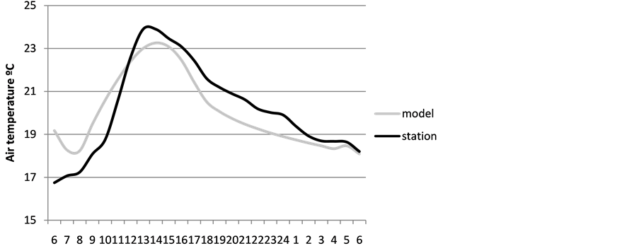
Figure 7 shows the measured temperatures and those supplied by the almost coincident model with a small difference at the beginning of the simulation. This may happen due to the fact that the simulation takes only 24 hours, since it is known that the model has limitations for the initial hours.
Figure 7(b) shows the temperature variation in a period of 24 hours starting at 6 a.m. on 08/01/2008 and ending at 6 a.m. on 08/02/2008. It follows the temperature variation for different patterns of land use, i.e., the actual area, an area with grass and an area with grass and tree. It is noteworthy that the point on the asphalt sur
 (a)
(a)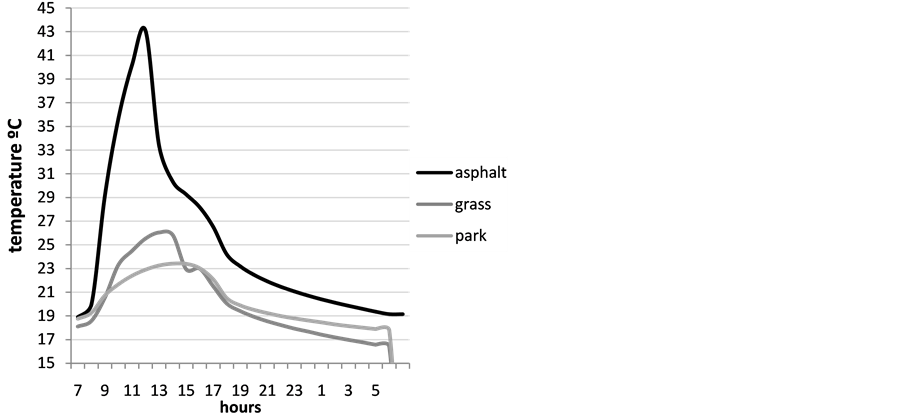 (b)
(b)
Figure 7. (a) Evolution of the temperatures measured by the Water Service and Sanitation Provider (SAE) and obtained by the model from 08/01/2008 to 08/02/2008; (b) Graph of the evolution of air temperature at the study spot within 24 hours.
face presented the highest temperature (43.0˚C) at noon. This temperature is associated with the irradiative property of the material (asphalt), which has average albedo of 0.20 and emissivity of 0.90 (figures in the data model) and lack of vegetation. The sandy soil of the study area has albedo of 0.30 and emissivity of 0.90. This point also presented the highest minimum temperature of 19˚C, so the temperature variation at this point was 24.0˚C within 24 hours simulation.
The simulation called “grass” showed maximum temperature slightly above 25.0˚C, at 2 p.m. on the study point (P), very below the maximum temperature on the asphalt (43.0˚C). At this point, the lowest minimum temperature was found to be 16.5˚C at 5 p.m., together with the grass/tree simulation point. The grass and grass/tree simulations showed higher emissions of long wave radiation, thus justifying the lower minimum temperatures. At this point, the temperature variation was 8.5˚C.
The structures containing trees, park and grass/tree presented the highest temperatures, at 2 p.m., 23.4˚C and 22.5˚C. There was a difference of almost 1.0˚C between these two simulations that can be explained by the difference in emissions of long wave radiation.
The grass/tree condition presented the lowest maximum temperature of 22.5˚C, the lowest minimum temperature of 16.5˚C and the lowest temperature variation within 24 hours, which was 6.0˚C.
Figure 8 shows the specific humidity evolution within 24 hours for four land uses. This specific humidity pattern is linked to the release of latent heat, thus the greater the release of latent heat, the greater the amount of steam in the atmosphere. The spot of the study simulation program showed the highest specific humidity, 20 g/kg and the greater release of latent heat 298 W/m2 at 1 p.m., followed by the spots located in park and grass/tree areas, 17.6 and 16.9 g/kg respectively. The spot located on the asphalt presented the lowest moisture that was specific to 11 g/kg at 2 p.m. The study point showed the highest specific humidity, 20 g/kg and greater release of latent heat 298 W/m2 at 1 p.m. followed by points located in the park and grass/trees areas, with 17.6 and 16.9 g/kg, respectively. The point located on the asphalt showed low specific humidity, with 11 g/kg at 2 p.m.
The specific humidity is linked to the latent heat release pattern in four simulated areas where the greatest release of latent heat leads to the highest amount of water vapor in the atmosphere. Thus, the point of simulation study called “grass” showed the highest specific humidity, 20 g/kg and the greatest release of latent heat 298 W/m2, at 1 p.m. followed by points located in Park and grass/tree simulations. The spot located on the asphalt showed specific humidity 11 g/kg at 2 p.m.
Thermal comfort values within the limits required by ISO 7730 submitted by the PMV and PPD indexes were found in only three situations, on the asphalt at 3 p.m., grass surface at 9 a.m. and park area at 3 p.m., as can be seen in Table2
The temperatures within the study points when thermal comfort was reported were: t = 29.0˚C in the paved area and t = 23.3˚C, both in the park at 3 p.m. and t = 20.5˚C, morning at 9 a.m. (grassy area).
Thermal comfort values within the limits required by ISO 7730, submitted by the PMV and PPD indexes were found in only three situations, on the asphalt at 3 p.m., grass surface at 9 a.m. and park area at 3 p.m., as can be seen in Table2
Although the grass/tree situation had been out of ISO standards, the results were very close to comfort at 9 a.m. tending to cold and at 3 p.m. tending to hot.
The thermal comfort is closely related to wind speed, since this variable may lead to heat loss by evaporation and transport of heat by convection. Thus, the vegetation changes the wind flow, increasing or decreasing the comfort sensation, depending on the type and height of plants.
Figure 9 shows that the simulation point program has the highest wind speeds, followed by grass/trees, park and asphalt situations, with 0.76, 0.61, 0.21 and 0.06 m/s, respectively.
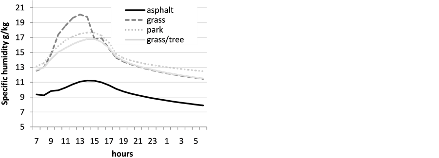
Figure 8. Graph of the specific humidity evolution at the study spot within 24 hours.
Table 2. Location of points within the grid and PMV and PPD values for each point at 9 h 00 min and 15 h 00 min.
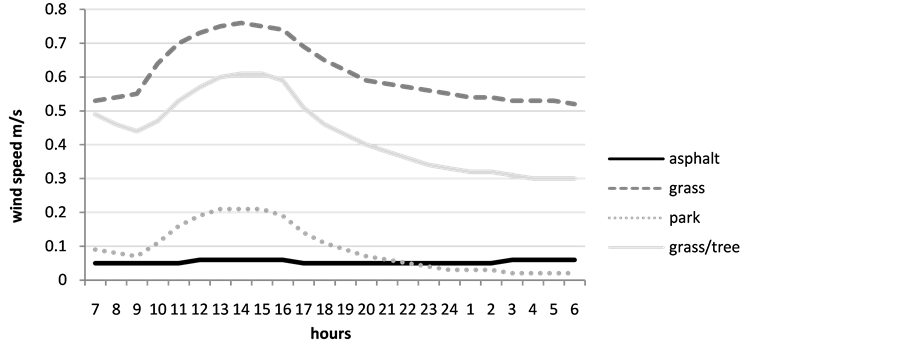
Figure 9. Graph of the wind speed at the soil surface.
The site roughness must be taken into account in the wind speed analysis. Thus, the wind speed is higher on the grassy surface compared to that of paved surface, since it is located in a distinct region near a building 10 m high and the other simulations rely on trees as a wind barrier and the incident radiation attenuation.
The wind speed variation within 24 hours was higher in the grass/tree simulation, with v = 0.31 m/s, although not presenting the highest speed.
The amount of energy seen on the top of the model, 2500 m above sea level is the same for all simulations. The differences are determined by the thermal properties of each situation analyzed, as the specific heat and thermal conductivity of the mulch, as well as the site roughness.
The energy balance is one of the most important determinants of microclimates and depends on the nature of the surface and the heat transport capacity of soil and atmosphere.
The energy balance is one of the most important determinants of microclimates and depends on the nature of the surface and the soil and atmosphere heat transportation capacity. By changing the soil nature, the capacity to absorb and release heat is also changed, increasing or decreasing the energy flow within the open land/atmosphere system (for energy exchange).
Figure 10 shows the short-wave radiation flow that interacts with the vegetation and soil surface at the study points within the grid for each type of surface. For the calculation of this radiation flux, the model uses an attenuation coefficient calculated from a foliar area index in 3D and the atmosphere extinction coefficient.
The point located on the asphalt showed maximum flow of direct radiation of 1400 W/m2 at noon, a higher value when compared to the other surfaces, which was 500 W/m2, at the same time. This difference in values can be explained by the influence of the existing vegetation, reducing the radiation flow.
In the park, the study point presents two hours of insolation (the total time interval between rising and decline of the solar disk was not hidden by clouds or atmospheric phenomena of any kind, Varejão, 2006), ranging from 11 a.m. to 1 p.m. To the point located on the grass area, this flow starts at 8 a.m. lasting 8 hours and finally to the point at the grass/tree surface, the insolation lasts 6 hours, starting at 10 a.m. So, the points located within areas with vegetation have the same amount of irradiative shortwave (500 W/m2) at different time periods depending on the shading caused by elements at the surrounding points.
The points located within grass/tree and park areas also suffer the effect of shading as can be seen in Figure 10, where the radiation is reaching zero after 1 p.m. The grassy surface receives direct radiation for longer time and tends to zero at 4 p.m.
Figure 11 shows the emission of long-wave radiation by the different surfaces under study. The spot on the asphalt that presented the highest short-wave radiation flow also showed higher emission of long-wave radiation, causing further warming of the atmosphere and having the highest temperatures. The response time of temperature increase by radiation was lower in the asphalt, where most short-wave radiation received and the maximum temperature occurred at 12 o’clock and can be explained by the high emissivity of the asphalt. The response time of temperature increase due to radiation was shorter in the asphalt, where most of the shortwave radiation received and the maximum temperature occurred at noon and can be explained by the high emissivity of the asphalt.
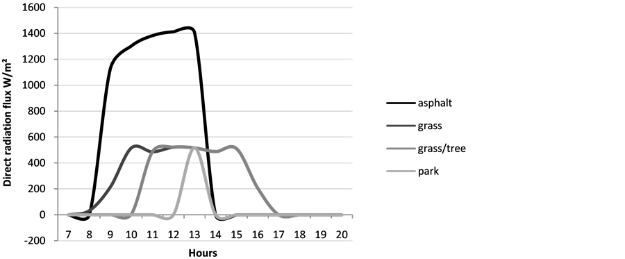
Figure 10. Flow of direct radiation at the study spot on 08/01/2008.
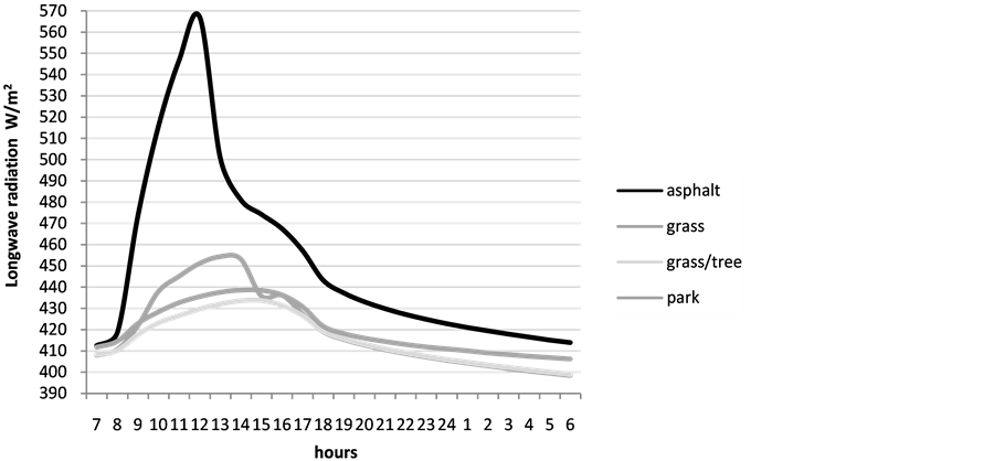
Figure 11. Long wave radiation emitted by the surface at the study spot on 08/01/2008.
The grassy, park and grass/trees areas showed the maximum temperatures at 1 p.m. and 2 p.m. respectively, i.e., 1 to 2 hours after the maximum radiation received. Although the reception of direct solar radiation ceases between 1 p.m. and 4 p.m., the radiation emitted by the surface remains after the 6 p.m., keeping air temperatures between 15.0˚C and 19.0˚C at the study spot.
Figure 12 and Figure 13 refer to sensible and latent heat flow at the study spot for different surfaces. The asphalted area released a large amount of sensible heat, compared to the grassy and trees areas (Figure 12). Sensible heat is the energy used to increase the mean temperature. Thus, the energy released at the study spot on the asphalt is being used to warm the environment, elevating the temperatures at this point. The transformation of radiant energy into sensible heat flux found on the asphalt surface showed maximum value of 670 W/m2.
Figure 12 and Figure 13 show the flow of sensible and latent heat at the study spot for various surfaces. The area covered with asphalt released large amount of sensible heat (673.37 W/m2 compared to grass (48.77 W/m2)), grass/trees (0.20 W/m2) and Park (5.35 W/m2) as shown in Figure 12. Sensible heat is the energy used to raise the average temperature. Thus, the energy released on the asphalt is being used to heat the environment, increasing its temperature at this spot.
The surface with grass showed higher latent heat values (Figure 13), compared to other coverings. This means large amounts of energy to convective processes in grass cover, because grass retains more humidity than asphalt.
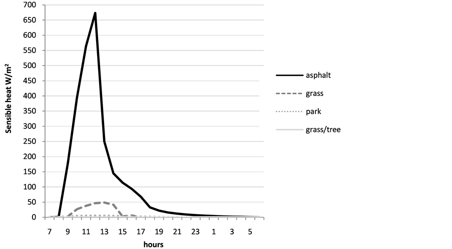
Figure 12. Graph of the sensible heat flow at the study spot for the different surfaces.
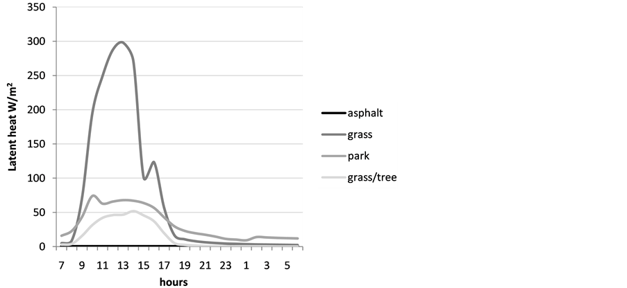
Figure 13. Graph of the latent heat flow at the study spot for the different surfaces.
The latent heat values obtained from the grassy surface was 300 W/m2. This represents less than half the sensible heat values released by the paved surface, showing that, in the region, the main heat transfer occurs by sensible heat flow. One of the main differences between rural and urban areas, according to OKE (1982), is that in rural areas, more heat is lost through evaporation (latent heat). In the cities, most of the heat transfer takes place by sensitive heat or due to soil sealing.
Surfaces with vegetation as high as 1 m produce mutual shading hindering the influx of solar radiation and resulting processes such as evapotranspiration. Convective processes are present in these simulations. With the presence of vegetation, the energy is used to change state and transport of steam to the atmosphere, causing a lowering in the temperature. With the presence of vegetation, the existence of heat and humidity uses energy for the change of state or transport of steam to the upper atmosphere, causing cooling in the environment. Thus, lower temperatures for areas with trees are shown in Figure 7.
When air temperature increases, there is a reduction in latent heat loss (by convection and radiation) making a living organism to increase its elimination through evaporation. Saturated air does not allow evaporation, causing people in these sites to have their temperature increased, when it is below the air temperature. If the air has low relative humidity, heat gain does not occur.
Thus, the asphalted environment with higher temperatures should be an area of greater discomfort for pedestrians. Nevertheless, this did not occur as shown on Table1 This thermal comfort shown in the asphalt spot can be explained by the shading effect occurring at 3 p.m.
4. Conclusions
The structures showing thermal comfort within ISO 7730 standards were the grassy area with no trees at 9 a.m., paved areas and park at 3 p.m. The spot within the asphalted area presented comfortable PMV and PPD indexes, i.e., MV = 0.5 and 10% of people dissatisfied with climatic condition in terms of shading caused by constructions. Although other cases have presented PMV and PPD indexes off the limits required by rules, they were very close to these values. The only spot having a far cry from the comfort was the spot in the asphalt at 9 a.m. The point on the asphalt was outside the limits of comfort at 9 a.m.
The results presented in this work show the importance of local architecture and land covering in this study area, which influences energy balance, wind speed, temperature and hence the thermal comfort. The presence of green areas is essential so that the population may enjoy the pleasant surroundings, both in work hours and in leisure time.