1. Introduction
The goal of stable isotope mixing models or “sourcing” is to estimate the proportional contributions of sources to a mixture. Stable isotope sourcing models are increasingly used to study animal diets and foodwebs, water sources in soils, plants, or water bodies, geological sources for soils or marine sediments, decomposition and soil organic matter dynamics, tracing animal migration patterns, evaluating management scenarios, and forensics [1] -[5] . Because animal ecology offers a rich complexity as a result of the preferential assimilation of elements from given sources into different tissues, we focus our attention here. The model, however can be applied widely. Stable isotope analyses of a consumer tissues (the mixture) and their potential prey and diet items (the sources) are a powerful and well-studied means of quantifying relative contributions of isotopically distinct dietary components providing many benefits in comparison with traditional methods for quantifying diet, such as the analysis of stomach and fecal contents [4] .
We introduce an algorithm and software, SISUS, for providing feasible source proportions of biomass consumed by a mixture using mass-balance mixing models. Our probabilistic method (SISUS) is preferred to the deterministic method (IsoSource [1] ) because it quickly and randomly samples a user-specified number of exact solutions from the solution polytope. In Section 2, we describe the model, illustrate the geometrical relationship between isotopic ratio space and the solution polytope, and describe the competing methods to sample the solution polytope. Section 3 describes the SISUS software. Section 4 provides results of a simulation study and an example. In Section 5, we discuss interpretation of results.
2. Material and Methods
2.1. Mixing Models
The isotope ratio,  , is a normalized ratio of the number of rarer to common isotopes in a sample,
  , relative to an international standard,
  , given in parts per thousand (per mil, ‰) [6] . Carbon and nitrogen are among the most commonly used elements for diet sourcing.
The basic mixing model (BMM) is the simplest mass-balance mixing model. It assumes that the mean isotope ratio of the mixture equals the diet-weighted average of the mean discrimination-corrected isotope ratio composition of the sources [2] [7] [8] . Assuming that  isotopes are measured and the consumer's diet consists of
  sources, the defining equations can be written as
 (1)
(1)
Coefficient  is the mean isotope ratio for isotope
  in the mixture. Each
  is the isotope ratio for isotope
  from source
 ,
,  , corrected by the addition of the discrimination,
 . Discrimination is the difference of the isotope ratio in the diet source from the isotope ratio in the mixture's tissues as elements are ingested, excreted, or catabolized (e.g., trophic fractionation, [9] [10] ). Mean diet
  is a vector restricted to the simplex, that is, each
  is nonnegative and the sum of the source proportions is 1. In practice
  and
and  are estimated from data, an issue that we address in Section 5.
The extended mixing model (EMM) increases realism by recognizing that both consumer and sources exhibit variation, and that elemental concentration and assimilation efficiencies of consumers for different food types can vary considerably [3] . The EMM has the same linear form as the BMM, thus the discussion applies to this more general model. Here we restrict our attention to the BMM.
2.2. Alaskan Bear Example
The summaries in Figure 1 reconstruct data from ([11] : Table 1). The goal is to determine the biomass contribution of salmon, terrestrial meat, and fruit to the diet of an average brown bear (Ursus arctos) from the Kenai Peninsula, Alaska, at a particular time of year [12] . Mean carbon and nitrogen isotope ratios are available from a sample of brown bear consumers, from samples of the three diet sources, as well as for the discrimination (i.e., difference between the consumer and each diet item) established from captive experiments. Figure 1 plots the discrimination-corrected isotope measurements for carbon/nitrogen pairs,  , for the three sources and mean carbon/nitrogen isotope ratio responses
  for brown bears. The isotope ratio data plot also includes the “convex hull” obtained by connecting the outermost sources with line segments. The data presented in Figure 1 can be described by the following matrix (2):
 (2)
(2)
The first row represents the equation for carbon, the second row is for nitrogen, and the third row is for the probability vector simplex constraint. The first column is for salmon, the second column is for meat, and the third column is for fruit. One or more solutions to (2) exist(s) if and only if the mean isotope ratio for the mix-

Figure 1. Convex hull plot of the Alaskan brown bear example. This plot represents the isotope ratio data space of discrimination-corrected carbon and nitrogen isotope ratios.
ture brown bear is not outside the convex hull, as shown in this example. Typically, the closer the isotope ratio values of the mixture are to a source’s discrimination-corrected isotope ratio values, the more similar the mixture is isotopically to that source, and the larger the contribution of that source can be to the mixture. Using both carbon and nitrogen, the solution for  in (2) is unique. The BMM estimates that brown bear tissues were derived (sourced) from 0.59 salmon, 0.10 meat, and 0.31 fruit. Both frequentist and Bayesian methods are available for estimation for unique solution situations [13] [14] .
Relationship between Data Space and Source Proportion Solution Spaces
In most studies the number of diet sources exceeds the number of isotopes plus one,  , leading to an infinite number of solutions to the BMM. The goal is to represent the solution space, or alternatively, to provide a set of “typical” solutions to the BMM. If
  as in the brown bear example, there is at most one feasible solution.
The data consists of  discrimination-corrected isotope ratio means on each of
  sources, thus, the isotope ratio data space is
  -dimensional while the source proportion solutions,
  are
are  -dimensional. Each of the linear equations in (1) defines an
  -dimensional hyperplane in the proportion solution space. Assuming
 , the intersection of the simplex and these hyperplanes is an
  -dimensional convex polytope. This convex polytope defines the set of solutions to the BMM.
In the brown bear data the  -dimensional isotope ratio data space in Figure 1 maps to the
  -dimensional proportion solution space in Figure 2(a). The solution space axes represent biomass contributions of each source,
  ,
,  , and
, and . The simplex equation is represented by the equilateral triangular plane in Figure 2(a). The gray plane heading back and up is given by the carbon equation, and the blue plane heading downwards is given by the nitrogen equation. The solution polytope is the intersection of the three planes, the point labeled “solution” at (0.59, 0.10, 0.31). If we considered carbon only, then the solution polytope would be the intersection of the carbon and simplex planes, that is, all points on the line segment joining c1 to c2.
2.3. Algorithms for Feasible Solutions
2.3.1. Approximate Solutions Using IsoSource
IsoSource is a popular deterministic algorithm used in stable isotope sourcing to represent the solution polytope from underconstrained linear mixing models where  [1] [15] . IsoSource evaluates a user-specified uniformly-spaced lattice of points on the simplex, labeling a point a solution if it satisfies the BMM within a userspecified tolerance. These are points on or close to the solution polytope, consistent with all possible solutions being equally likely a priori. This is a brute force strategy because no information is used regarding the location of the solution polytope within the simplex. For a fixed tolerance, decreasing the increment of the grid space hyperexponentially increases the number of points evaluated, increasing both the number of solutions returned
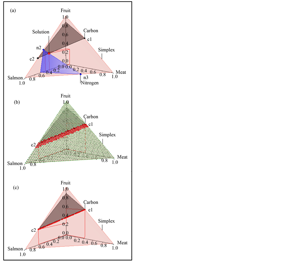
Figure 2. BMM Alaskan brown bear example. (a) Solution space using both carbon and nitrogen. (b) Using carbon only, IsoSource evaluates points on the lattice over the simplex, returning 114 approximate solutions of the 1326 evaluated points. (c) Using carbon only, SISUS samples 114 exact solutions uniformly over the solution polytope.
and the time for the algorithm to execute. For a fixed increment, decreasing the tolerance increases the accuracy of the solutions by excluding points far from the solution polytope. Because the number of approximate solutions depends on the size of the solution polytope, the increment grid spacing, and the solution tolerance, it may be challenging to choose settings to balance the desire for many solutions, accurate solutions, and acceptable execution time.
Figure 2(b) illustrates the IsoSource sampling strategy, applied to the carbon-only brown bear example with a grid increment of 0.02 and tolerance of 0.10 where 114 of the 1326 points evaluated are approximate solutions. The points evaluated are uniform over the simplex, but the approximate solutions provided are only roughly uniform near the solution polytope.
2.3.2. Exact Probabilistic Solutions via SISUS
SISUS implements a two-step algorithm to sample exact solutions uniformly from the solution polytope. The first step is to determine the vertices and boundaries of the solution polytope. The method is complex to describe [16] , but is already implemented [17] . The second step is the probabilistic sampling from the solution polytope, using the random directions symmetric mixing algorithm [18] [19] . There are three steps in this algorithm: (0) Choose a starting point inside the solution polytope,  , and set counter
 . (1) Generate a random direction
  uniformly distributed over a direction set inside the solution polytope
 , find the line set
 , and generate a random point
  uniformly distributed over
 . Descriptively, we draw a line segment through the current point
  to two edges of the polytope along the chosen direction, then generate the next point
  uniformly at random from that line segment. In this way we move around the polytope collecting a representative sample. (2) When we reach the desired number of samples,
  , the computation stops. Otherwise, the counter is incremented
  and the procedure is repeated from to step (1). The sample is generated rapidly and converges to a uniform distribution over the solution polytope [20] .
Figure 2(c) shows  exact probabilistic solutions from SISUS for the carbon-only brown bear example, which are qualitatively similar to the deterministic approximate solutions of IsoSource.
3. Software
SISUS uses the random directions symmetric mixing algorithm in R package polyapost, function constrppprob [21] -[23] . The number of sources  and isotopes
  may both be large, provided
 . Sample sizes of
  and 10000 appear reasonable for exploration and publication, respectively. Standard Markov chain Monte Carlo diagnostics are used to monitor convergence of the algorithm (sec. 11.11, [24] ), though convergence issues are extremely rare and are typically due to random sampling rather than algorithmic issues.
SISUS software is freely available at StatAcumen.com/sisus and as an R package at cran.r-project.org/web/ packages/sisus. Data and parameter settings are input into a single OpenOffice.org-compatible MicroSoft Excel 2003 workbook. This workbook is then either uploaded to the website for processing or processed by a local installation of the SISUS package in free statistical software R on Windows, Mac OSX, or Linux platforms. Specified samples, summary tables, and plots in a variety of requested image formats are returned.
4. Results
4.1. Execution Time, Solution Predictability, and Solution Accuracy
There are three reasons why the probabilistic approach (SISUS) is preferred over the deterministic approach (IsoSource). These are (a) the relatively short execution time, (b) the predictability of the number of solutions, and (c) the solution accuracy. In Figure 2 we already touched on points (b) and (c). We use a fabricated example to further illustrate the differences in these approaches. We analyze subsets of the problem
 (3)
(3)
The full problem has  sources and
  isotope ratios, as that is the extent of the problem size that IsoSource is programmed to solve. For each example, Table 1 specifies a given value for
  and
and , and the problem is defined by choosing the first
  columns and first
  rows plus the simplex constraint of (3). Table 1 reports the execution times for SISUS and IsoSource running on a PC (Dell Optiplex GX260 with Intel Pentium 4 2.40 GHz CPU with 512 MB RAM) without any additional significant processes running.
For SISUS we obtain  exact solutions for each problem size by finding 100R solutions and keeping every 100th to increase the independence of the samples and to improve solution polytope coverage.
From Table 1 it is clear that execution time for SISUS increases with  up to a few minutes while IsoSource increases to hours. For SISUS the time to obtain a specified number of exact solutions grows nearly linearly with the number of sources
  and quadratically with
 . For IsoSource an increment and tolerance are specified which determines a hyperexponentially growing number of iterations with
  given by the Binomial coefficient (Equation (3), and (1))
 (4)
(4)
Approximate solutions are then returned which are within the tolerance of exact solutions. Time scales roughly linearly with the number of iterations (about 1M/s). For small problems , IsoSource takes only a few seconds. But as the problem size increases, the time increases to hours. Two cases to note: a) For
 , as
, as  increases
  and the solution polytope decreases in dimension
  the solutions become more difficult to find for IsoSource resulting in fewer or no approximate solutions. b) The largest example,
  ,
,  ,
,  , finds only 1 approximate solution after almost 5 hours of computation, and larger increments fail to find any solutions. Setting the increment to 1 will increase the running time to roughly 68 days. In each of these cases, SISUS provides 10,000 exact solutions in less than 30 seconds.
4.2. Mink Example
We use published mink (Neovison vison) data [25] to further illustrate capabilities of SISUS. The BMM is given by
 (5)
(5)
where the rows are for carbon, nitrogen, and the simplex. The left vector is the mixture mink and the columns of the matrix are for the  sources of fish, mussels, crabs, shrimps, rodents, amphipods, and ducks. The convex hull of the discrimination-corrected sources includes the mink, thus there are feasible solutions. The solution polytope is a
  -dimensional object in
  -dimensional proportion space.
Figure 3 provides graphical summaries of the solution polytope returned by SISUS, based on 10,000 solutions. Time to compute the solutions is similar to that reported in Table 1 for  sources and
  isotopes. Marginal histograms of the 10,000 solutions for each source are given along the main diagonal. Two-dimensional histograms for each pair of sources are given above the main diagonal of the plot while corresponding pairwise density plots are provided below the main diagonal. The oneand two-dimensional histograms show that the marginal and pairwise solutions are highly constrained within the unit interval and unit square, respectively.
5. Probabilistic Interpretation and Discussion
IsoSource [1] , with nearly 1000 citations, is extensively used for inferences based on mixing models. The natural interpretation of the IsoSource solutions is as samples from the Bayesian posterior distribution of the vector  of mixture proportions. As the components in the BMM defined in (1) are estimated from data but treated as fixed by IsoSource, it can be shown that random samples from the solution polytope are an approximate sample from the posterior distribution of
 , assuming that the samples for estimating the isotope ratios and discriminations are large, and that the prior distribution for
  is uniform over the simplex. As SISUS generates random samples from the solution polytope rather than approximate solutions, we consider SISUS a better inferential tool. Thus in the mink analysis, the plots in Figure 3 summarize the univariate and bivariate large sample posterior distributions for the contribution of sources to mink diet. The samples may be used, for example, to estimate the posterior probability that Amphipods contribute to at least 10% of the mink diet, or to computing the (posterior) means for each proportion, which is a point estimate of the contribution of a source to the diet. Table 2 lists the posterior means and standard deviations for each source in the mink example. The SISUS large sample analysis suggests that fish comprises approximately 0.67 of mink diet, with each of the remaining six sources contributing to roughly equally.
The mink data set is small, with sample sizes ranging from 5 to 25 with an average of 11.3, so it is important to gauge the utility of this SISUS analysis relative to a complete, but more complex, Bayesian analysis. Several
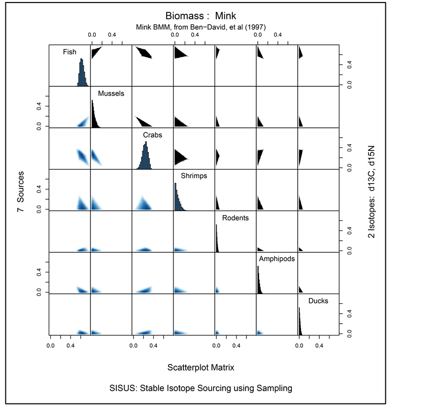
Figure 3. Mink BMM example marginal histograms along diagonal, scatter plot of paired source contributions on the upper diagonal, and corresponding two-dimensional density histograms on the lower diagonal.
researchers have developed Bayesian models for inference using the BMM [26] -[28] . These models are somewhat restrictive as they assume that the source isotope ratios or discrimination are estimated without error, or that the multivariate isotope ratio data have independent components. For a realistic assessment of SISUS, we considered a Bayesian model for the mink data that assumes independent multivariate normal distributions for correlated isotope ratio responses from the mink mixture, the seven sources, and for estimating discrimination from two diet experiments [14] . In a second Bayesian analysis, we considered the effect of tripling the sample sizes but keeping all other sample summaries the same. Diffuse but proper prior distributions were used throughout.
Table 2 gives estimated posterior means and standard deviations for the seven components of mink diet. One analysis uses both isotopes. The other two analyses consider carbon and nitrogen separately. Considering the analysis based on the original data, the posterior means based on SISUS tends to identify the major and minor sources of mink diet, but the estimates of the dominant sources are somewhat inaccurate. The SISUS summaries also tend to underestimate uncertainty in the marginal posterior distributions, which is expected. The SISUS means and standard deviations for analyses based on a single isotope are much more accurate, as are the summaries for analyses in which the sample size was tripled.
We find that in general SISUS produces a simple approximate assessment of the mean proportion in the

Table 2. Selected numerical summaries for the mink example based on SISUS, fully Bayesian analyses, and Bayesian analyses with triple the sample size. Values represent feasible source contributions of biomass to mink.
BMM and EMM but tends to underestimate uncertainty. In our opinion, SISUS is especially useful for secondary analyses of published data and in settings where individual level data needed for a complete Bayesian analysis may not be available.
Acknowledgements
EBE thanks Keith Hobson for initial support during this project.