1. Introduction
In 2008, the world experienced a dramatic surge in the prices of commodities. The prices of food commodities, in particular maize, rice and wheat increased dramatically from late 2006 through to mid-2008, reaching their highest levels in nearly thirty years. Prices stabilized in the summer of 2008 and then decreased sharply in the midst of the financial and economic crisis [1] . A similar price pattern emerged in early 2009 when the food commodity price index slowly began to climb. After June 2010, prices shot up, and by January 2011, the index of most commodities exceeded the previous 2008 price peak [2] . Sharp increases in agricultural prices are not uncommon, but it is rare for two price spikes to occur within 3 years as they normally occur with 6 - 8 years intervals. The short period between the recent two price surges has therefore drawn concerns and raised questions. What are the causes of the increase in world agricultural prices and what are the prospects for future price movements? Will the current period of high prices end with a sharp reversal as in previous price spikes, or have there been fundamental changes in global agricultural supply and demand relationships that may bring about a different outcome?
A number of authors have discussed the factors lying behind the spikes though no agreement has been reached on the cause of these phenomena. Rapid economic growth in China and other Asian emerging economies, decades of underinvestment in agriculture, low inventory levels, poor harvests, depreciation of the US dollar, and speculative influences are some of the factors considered and cited as leading to high levels of commodity prices [3] -[5] . In addition, the diversion of food crops as bio-fuels stands out as an important and new factor that many have seen it as accountable for the food price spikes [6] .
The recent price spikes were also accompanied by volatile commodity prices. There is evidence of increased price volatility from mid-2000 for most food commodities in particular those of grain prices [7] . Price volatility in commodities has been considerable, making planning very difficult for all market participants. Sudden changes and long run trend movements in agricultural commodity prices present serious challenges to market participants and especially to commodity dependent and net food importing developing countries. At the national level, food-importing countries face balance-of-payment pressure as the cost of food imports rise. When transmitted to domestic markets, high world prices erode the purchasing power of urban households and other net food buyers. Poor urban households are particularly affected because they spend a large share of their income on food [8] .
A majority of analyses examining biofuels impacts on energy and food commodity markets have focused the attention on price-level links while price volatility has received much less attention. An increased correlation between food and energy prices is likely to yield stronger volatility spillovers between prices in these two markets. The recent 2007/08 crisis has stimulated research in the area of commodity price volatility, which can usefully complement the larger body of research which looks at price level impacts.
Previous research has shown that in the recent decade there has been an increase in volatility grains, vegetable oils and meats [9] . These are commodities which are likely to be affected by the growth of biofuel production. On this view, heightened food price volatility arises due to the importation of oil price volatility. Despite this, crude oil price volatility has not been particularly high over the period considered. This suggests that the relationship between crude oil and grains prices may have changed over the most recent decade resulting in a greater transmission of oil price volatility into grains prices. Consistent with this view, grains and crude oil returns have in the recent years been co-moving as shown by the increased correlations between the two groups [10] . These increased correlations may be accounted for either in terms of an increase in the pass-through from the crude oil market to the grains markets or by an increased prevalence of common shocks across the two sets of markets.
The objective of this paper is to analyze the cause of increased food commodity volatility. We investigate whether the volatility in food commodities is now driven by the transmission of shocks from the crude oil market as a result of increased biofuel production and consumption. We employ Multivariate General Autoregressive Heteroskedasticity (MGARCH) models which have mainly been used hitherto in the analysis financial market data. Using estimates from the Dynamic Conditional Correlation (DCC) Multivariate GARCH models [11] specification, we decompose volatility of food commodities into its main components. Conditional correlations are calculated from MGARCH models estimated on daily data over the twelve-year sample 2000-2011. Increased commodity comovement implies a rise in inter-commodity correlations. An advantage of the DCC framework is that it allows us to focus specifically on changes in pass-through from the crude oil market to the grains markets. We therefore pose the hypotheses of interest within the DCC multivariate GARCH model [12] .
2. The Relationship between Food and Energy Commodities
Crude oil prices can affect the prices of food commodities in two distinct ways. First, crude oil enters the aggregate production function of most primary commodities through the use of various energy-intensive inputs such as fertilizers, heating and pesticides and through transportation costs. However, agriculture is not highly energyintensive so this impact is will not be large and there is no reason to suppose that it has increased markedly in recent years.
Secondly, some food commodities can be used to produce substitutes for crude oil. This is true in particular of maize and sugar cane in ethanol production and oil seed rape and other vegetable oils for biodiesel production [13] . The attractiveness of production of ethanol and biodiesel, and of the investment in refining capacity to produce these products, depends directly on the price of crude oil. One should thus expect to find a relationship between food commodity prices and crude oil prices. Although the impact of higher crude prices on the demand and supply of grains and oilseeds takes time, efficient futures markets should anticipate these effects.
It is useful to distinguish the price level and price volatility effects of the expansion of biofuels production. The former arises through the diversion of supplies from food and feed consumption. This happens directly via competition between food and feed users and biofuel users for the same grain, but also indirectly, through the substitution of one grain, such as maize diverted to biofuel feedstock from use as food or feed rations, leading to substitution of a food grain, such as wheat, into animal feed. Soybeans are most directly affected by the demand for corn-based ethanol as corn and soybeans tend to compete for land area and can be used in rotation.
The US expanded maize (corn) area by 23 percent in 2007 in response to high maize prices and rapid demand growth for maize for ethanol production. This expansion resulted in a 16 percent decline in soybean area which reduced soybean production and contributed to a 75 percent rise in soybean prices between April 2007 and April 2008. The expansion of biodiesel production in the EU diverted land from wheat and negatively affected wheat production and stock levels. This was in response to the increased demand and rising prices for oilseeds, land cultivated for oilseeds—particularly rapeseed—increased. Oilseeds and wheat are grown under similar climatic conditions and in similar areas and most of the expansion of rapeseed and sunflower displaced wheat or was on land that could have been used for wheat cultivation [13] . Grains prices also affect the price of meat and dairy products because grain is used as feed. Livestock feeding is the largest single use of corn and cattle, pigs and poultry all use corn feed.
The second effect of biofuels is it may increase the volatility of food prices. Gilbert and Morgan note that the volatility of any commodity price depends on the variances of shocks to production and consumption in conjunction with the elasticity of supply and demand. Within this framework, the biofuels link may be seen as introducing an additional source of demand variability and, if biofuel mandates are inflexible, may decrease demand elasticities. The main focus of the current paper is on these volatility links.
The direct production function link from crude oil prices to energy prices is well-documented. Using different methodologies, Baffes (2007) and Gilbert (2010) agree in seeing an energy price pass-through to grains prices of between 15 and 20 per cent. It is unlikely that this has changed over recent years. The indirect links, via the use of food commodities as biofuel feedstocks, are more difficult to quantify, in part because of the shortness of the relevant biofuels time series. Moreover, few of the formal models have been able to accurately capture the cross-commodity supply and demand linkages between corn—the primary grain used to make ethanol—and other commodities such as soybeans, wheat, and other feed grains. This motivates an examination of whether there has been a change or evolution of the relationship between food prices and the crude oil price over the period in which biofuels production has become important.
Gilbert used Granger-causality (GC) tests to examine the link between crude oil prices and both the IMF’s agricultural food price index and a grains sub-index [14] . In both cases, his results showed a negative impact Granger-causal in the two decades up to 1989 and a positive Granger-causal impact in the two more recent decades. The pre-1989 results may reflect the fact that, over that period, the developed economies lacked a clear monetary anchor and hence a rise in oil prices would likely be met by a tough anti-inflationary monetary tightening. The production function pass-through-impact of higher oil prices only becomes apparent once the credibility of inflation targeting had been established.
Tyner confirms that since the ethanol boom took off in 2006, the correlation between energy and agricultural markets has been strong. He highlights the summer of 2008 as the period where these two markets were closely linked. As the crude oil price increased so did the price of corn and other agricultural commodities. And when crude oil prices started to decline after the summer of 2008, so did the prices of most agricultural commodities. He highlights the blending wall as the determinant to this link. This factor is particularly influential in the case of high crude oil prices. Since ethanol production is limited by the blending wall, when crude oil prices are high, and the corn price increase is dampened. Thus the crude-corn price link that has been established could be significantly weakened at high crude oil prices because of the blending wall limit [15] .
The hypothesis of interest is therefore that increased biofuels production resulted in a higher pass-through coefficient from crude oil to grains prices. If this hypothesis is true, then crude oil price volatility will have had a greater impact on grains price volatility than previously even though the volatility of crude oil prices did not itself increase.
3. Effects of Biofuels
Global biofuels production has increased rapidly over the last 20 years. In the US, biofuels production started to rise rapidly in 2003 while in the EU it accelerated from 2005. The US expanded maize area by 23 percent in 2007 in response to high maize prices and rapid demand growth for maize for ethanol production. This expansion resulted in a 16 percent decline in soybean area which reduced soybean production and contributed to a 75 percent rise in soybean prices between April 2007 and April 2008. The expansion of biodiesel production in the EU diverted land from wheat and negatively affected wheat production and stock levels. This was in response to the increased demand and rising prices for oilseeds, land cultivated for oilseeds—particularly rapeseed—increased. Oilseeds and wheat are grown under similar climatic conditions and in similar areas and most of the expansion of rapeseed and sunflower displaced wheat or was on land that could have been used for wheat cultivation [16] .
This expansion in biofuels production, particularly in the United States and Brazil, has been driven by a number of economic and environmental factors. High crude oil prices and keenness to promote non-petroleum energy sources to reduce dependence on oil imports have fuelled interest in the United States, Brazil, and the European Union in finding alternative energy sources. Environmental concerns about greenhouse gas emissions and the urge to slow down global warming due to fossil fuel emissions have also contributed to the expansion [16] . Despite these diverse motivations for the alternative energy, there is still a debate on the factors that led to the boom in the ethanol industry from middle of the recent decade. Some authors believe that the boom was mainly driven by the market and in particular by the increase in crude oil prices. Others sustain that the boom was mainly driven by government policies, such as mandates, tax credits and the blending wall in the US aimed at increasing energy self-sufficiency and at reducing emissions in Europe [17] .
Increased biofuel production has sparked mixed reactions leading to what some have called the “food versus fuel debate”. Some commentators highlight the repercussions and risks which may result from increased reliance on biofuels. Increased biofuel production has increased the demand for feedstocks. This demand is mainly satisfied by grains and vegetable oils and this in turn may have increased the prices of these food commodities.
Biofuels have two main distinguishable effects. The first effect is that diversion of food crops into biofuels production raises the price levels due to diversion of supplies from food and feed consumption. This happens directly via competition between food and feed users and biofuel users for the same grain, but also indirectly, through the substitution of one grain, such as maize diverted to biofuel feedstock from use as food or feed rations, leading to substitution of a food grain, such as wheat, into animal feed. Soybeans are most directly affected by the demand for corn-based ethanol as corn and soybeans tend to compete for land area and can be used in rotation.
Grains prices also affect the price of meat and dairy products because grain is used as feed. Livestock feeding is the largest single use of corn and cattle, hogs, and poultry all use corn feed, thus the expansion in the ethanol industry does affect livestock production. Prices will adjust quickly for some such as chicken, milk and eggs, but take more time for others such as beef and pork. The price adjustment period reflects the length of time farmers need to adjust their stock (supply) in response to the higher feed prices.
The second effect of biofuels is it may increase the volatility of food prices. Gilbert and Morgan (2010) note that the volatility of any commodity price depends on the variances of shocks to production and consumption in conjunction with the elasticity of supply and demand. Within this framework, the biofuels link may be seen as introducing an additional source of demand variability—see Wright (2011) who emphasizes the transmission of energy market shocks into food commodity markets—and, if biofuel mandates are inflexible, as decreasing demand elasticities. The main focus of the current paper is on these volatility links.
4. Volatility in Food Commodity Prices
An increase in food commodity price volatility can be due to one or more of the following four factors:
• An increase in the variance of demand shocks; the diversion of food crops into biofuel production could lead to increased demand variability. Increased demand for food commodities, in particular corn, in the recent decade sugar and vegetable oils, as biofuel feedstocks has increased the correlation between agricultural prices and the oil price. This allows transmission of oil price volatility to agricultural prices, in effect increasing the variance of demand shocks;
• An increase in the variance of supply shocks; Poor harvests such as those experienced Australian wheat harvests in 2006 and 2007 and a poor European 2007 harvest have been mentioned as possible causes of the recent food price spikes. However, these poor harvests were offset by good harvests elsewhere in the world, notably Argentina, Kazakhstan and Russia, and 2008 harvests were good;
• A decline in the elasticity of demand; elasticity in demand depends on the response of consumers to price changes and this in turn depends on the price transmission i.e. the extent to which prices on world markets are passed through to local prices. Government interventions such as subsidies in response to higher food prices are diminish price responsiveness on the part of consumers thus rendering markets and prices highly inelastic. US government policy interventions through tax credits, mandates and subsidies have been identified as rendering corn and biofuel markets less responsive to changes in crude oil and gasoline prices;
• A decline in the elasticity of supply: Grain inventories have fallen over time since the millennium. Increased demand for corn and other feeedstocks for biofuel production have in turn reduced the responsiveness of supply to the demand shocks thus increasing volatility in these commodities.
Our analysis focuses on grains and, to a lesser extent, since these are overall the most important food crops. Grains are the major staple food across the globe and also are an input into the production of meat products. Moreover, grains were the main commodities that have been affected in the recent food spikes and are thus are crucial within the food price volatility question.
We examine the prices of:
• Maize (corn): The analysis of corn price volatility is for three reasons. First, maize (white) is a staple food in eastern and southern Africa. Second, it forms the main ingredient in animal feed in the United States. Third, it is the main biofuel feed stock in the United States;
• Wheat: It is the most important grain in temperate regions; in recent times it has been used as a substitute to maize in animal feed;
• Soybeans: It is important both as an animal feedstock and, when crushed, as a vegetable oil. It also competes for land with corn in the United States.
5. The Multivariate GARCH Framework
Bollerslev et al. (1988) provided a framework for multivariate GARCH (MGARCH) analysis. The general MGARCH (1,1) model for an m-dimensional vector r of returns is
 (1)
(1)
This representation is problematic if the dimensionality m of the return vector exceeds two, firstly because the model becomes highly parameterized—the number of parameters is —and secondly because it is difficult to impose positive definiteness of the conditional variance matrix Ht at every date in the sample. For these reasons, the literature has tended to work with simplified versions of the general MGARCH model.
Two radically simplified versions of the MGARCH model are commonly used. The first is the constant conditional correlation MGARCH (CCC-MGARCH) model introduced by Bollerslev (1990). In the diagonal case, this has the structure
 (2)
(2)
with . The scedastic Equation (2) may be written more compactly as
 where
where
 (3)
(3)
and  is a constant positive definite correlation matrix. This reduces the parameterization to
  (30 when m = 4) but the imposition of positive definiteness remains difficult except in the equicorrelation case in which
 where l is the vector of units.
The second widely used MGARCH model is dynamic conditional correlation (DCC) model of Engle (2002) defined by:
 (4)
(4)
where  is the unconditional variance-covariance matrix and a and β satisfy
  and
and . The conditional correlation matrix, which is now time-varying, is
 . This is a highly parsimonious specification—given the unconditional matrix
 , the model contains only 3 additional parameters. Positive definiteness is guaranteed by the inequality restriction on a and β.
It is apparent that the trade-off between the CCC and DCC MGARCH specifications is that CCC imposes a constant correlation structure but leaves the variance dynamics unrestricted across the difference returns while DCC allows a time-varying correlation structure but at the expense of imposing homogeneity of the variance dynamics. Depending on the context, one or other set of restrictions will be more appropriate. In our context, in which we are interested in the increased comovement of various commodity futures prices, we are obliged to choose the DCC route.
Consider a model for k > 1 commodity futures prices. Set crude oil as commodity 1 so that the remaining commodities are 2, …, k. The standard DCC model treats the k prices symmetrically so that Equation (4) states
 (5)
(5)
6. Grains Market Volatilities
In this section we report results relating to the comovement of the WTI crude oil price and the three principal grains and oilseeds traded on the Chicago futures market—corn, soft wheat and soybeans. Although only corn is directly used as a biofuels feedstock but the prices of the three grains move closely together as many north American farmers are easily able to reallocate land from one crop to another (in particular from soybeans to either corn or wheat) at the time of planting.
We use daily data for the front contract on the NYMEX WTI market and the CBOT corn, wheat and soybeans markets from 5 January 2000 to 30 December 2011. Prices are excluded for a small number of days on which one market was closed while the other traded. Contracts are rolled on the first day of the expiration month and returns are contract-consistent.
Throughout we estimate GARCH (1,1) models in conjunction with mean processes without any dynamic structure. Tests indicate that these specifications are adequate. Table 1 reports the univariate GARCH estimates and Table 2 the CCC MGARCH estimates. A standard likelihood ratio test gives a clear rejection of the univariate models against the CCC alternative and this is confirmed by the lower Akaike Information Criterion (AIC) for the CCC model. Inspection of the estimated coefficients show reduced heterogeneity in the ARCH and GARCH parameters in the CCC model relative to the univariate models. The estimated correlations between the three grains and WTI have a similar order of magnitude in the range 0.18 to 0.23. The inter-grains correlations are higher, around 0.62 for the wheat and soybean correlations with corn but 0.48 for the wheat-soybeans correlation. This suggests that corn plays the central role in the grains complex.

Table 1. Univariate GARCH estimates.
Sample: Daily, 5 January 2000 to 30 December 2011 (3001 observations); Robust standard errors in parentheses.
Table 2. Multivariate CCC-MGARCH estimates.
Sample: Daily, 5 January 2000 to 30 December 2011 (3001 observations); Standard errors in round parentheses (robust for coefficients); Tail probabilities in square parentheses.
Table 3 reports the Dynamic Conditional Correlations Multivariate GARCH estimates. The DCC MGARCH model is associated with the higher likelihood and lower AIC compared to the Univariate and CCC models and therefore appears to be preferred. We conclude that the DCC model is the preferred specification. We therefore henceforth focus on the DCC-MGARCH estimates.
Figure 1 shows the estimated correlations between crude oil and the three grains from the DCC MGARCH model and Figure 2 does the same for the inter-grains correlations. The correlations of the three grain price returns with WTI returns (Figure 2) moves from the 0.1 - 0.2 range in the first half of the sample to the 0.4 - 0.5 range in 2008-09. These correlations have subsequently fallen back but remain around 0.3. By contrast, the inter-grains correlations are higher, in the 0.4 - 0.6 range, but appear broadly constant through the sample.
These estimated correlations show considerable variability. After the text edit has been completed, the paper is ready for the template. Duplicate the template file by using the Save As command, and use the naming convention prescribed by your journal for the name of your paper. In this newly created file, highlight all of the contents and import your prepared text file. You are now ready to style your paper.
Table 3. Multivariate DCC-MGARCH estimates.
Sample: Daily, 5 January 2000 to 30 December 2011 (3001 observations); Robust standard errors in parentheses.
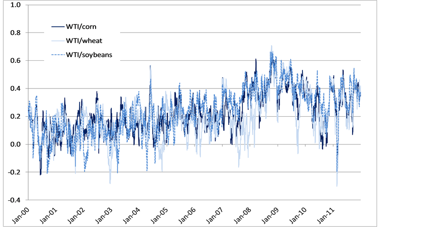
Figure 1. Estimated crude oil-grains correlations, DCC model.
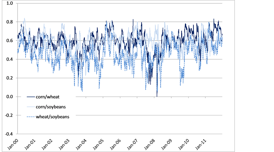
Figure 2. Estimated inter-grains correlations, DCC model.
7. Volatility Decomposition
The proposed decomposition model is based on the simple regression
 (6)
(6)
where:
 : logarithmic prices of corn, wheat and soybeans;
 : logarithmic price of crude oil;
 : idiosyncratic error.
First consider the standard representation in which the two coefficients  and
and  are constant over time. The result is a two-way decomposition.
The regression (6) is not proposed as structural or causal but is simply a means of obtaining the standard orthogonal decomposition of the variance of each price into a component which lies in the crude oil price space and one in the corresponding null space. We nevertheless interpret the  coefficients as measures of pass-through on the basis that the grains tail cannot wag the crude oil dog. However, it remains true that elevated
  coefficients may also reflect an increase in shock commonality.
We use the DCC-MGARCH model to allow  and
and  to evolve over time. This is comparable to, but not identical to, estimating regression (6) recursively or using a rolling window. It generates a third element to the decomposition arising out of the changing correlation between crude oil and grains prices.
This simple methodology therefore allows decomposing the conditional volatilities for corn, wheat and soybeans into variations in three main components:
• commodity specific volatility;
• crude oil volatility;
• the pass-through coefficient.
The conditional volatility for each of the three grains is therefore:
 (7)
(7)
We apply this decomposition to the DCC conditional variances discussed in the previous section estimating the pass through coefficients  by the ratio of the conditional grain-crude oil covariances to the conditional crude oil variance. Using the estimated DCC-MGARCH we conduct counterfactual decompositions for each of the grains conditional volatilities. From these estimates we are able to retrieve the three components. Estimate the average volatility values of 2000-05. We simulate the volatility components of each of the grains, holding constant the other components. In this way we are able to isolate the effects of each of the components over time.
The DCC-MGARCH model gives continuous estimates which can be comparable to a recursive regression. While the recursive regression estimates constant parameters over time. DCC-MGARCH model gives an estimate of evolving parameter over time (given that β < 1).
Figure 3 shows the volatility decomposition for corn. Corn volatility is dominated by idiosyncratic volatility. The gamma and crude oil volatility components remain relatively stable and insignificant from 2005. They become very significant from mid-2008 when crude oil prices are high. In particular the WTI-γ component that represents the pass-through coefficient of shocks from crude oil to corn rises in 2008. The high crude oil prices are transmitted into corn price volatility as both the “pass-through coefficient” beta and crude oil volatility are significant. Crude oil prices are important in explaining the 2008-09 increase in grains volatility.
Figure 4 reports the volatility decomposition over time for wheat. As in the case of corn, both the WTI-γ and WTI volatility components remain dormant from 2006 and then sharply rise in 2008. The idiosyncratic component is also relatively stable over time apart from two significant peaks. The first occurs in 2008 where droughts in the Australia and poor harvests in the European Union and Ukraine rendered wheat prices volatile. The second is in 2010 where the combined effects of a strong demand and fall in world wheat production increased volatility in wheat prices.
The soybeans volatility decomposition is represented in Figure 5. The idiosyncratic component of volatility is important and relatively stable over time. As in the previous cases, both the WTI-volatility and WTI-γ components are important in 2008 in explaining the conditional volatility of soybeans.
Table 4 looks specifically at the volatility impacts of changes in the pass-through coefficients  over the
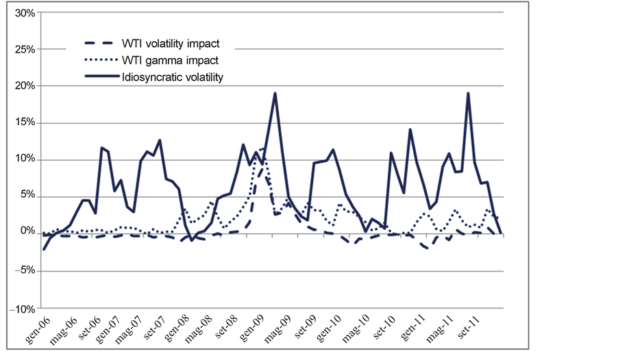
Figure 3. Corn price volatility decomposition.
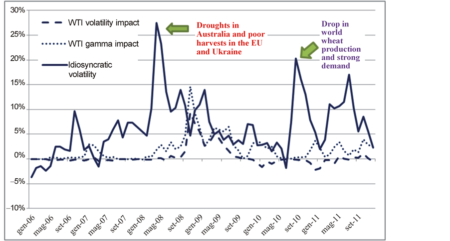
Figure 4. Wheat price volatility decomposition.
period of the food price spike and the financial crisis. The first three columns give actual conditional volatilities; the second block of three columns gives the counterfactual volatilities obtained by holding the pass-through coefficients γ constant at their average 2000-05 values; while the third block reports the differences.
The differences are all positive indicating that increased pass-through was seen as a contributory factor to higher grains volatility over this period. However, the effects are generally modest accounting for only around 2% - 3% of the 10% - 15% volatility increases. The single exception is the final quarter of 2008 when both crude oil and grains prices suffered a sharp fall. The impact of increased pass-through rises to over 10% The Tin this quarter.
Figure 5. Soybeans price volatility decomposition.
The table compares actual conditional volatilities (daily, converted to an annual rate) with counterfactual conditional volatilities holding the passthrough coefficients γ constant at their average 2000-05 values.
8. Conclusions
Food commodities prices have increased and become more volatile over the recent decade attracting the attention of market participants and policy makers. The short period between the recent price surges has therefore drawn concerns and raised questions on the causes and future prospects of commodity markets. Biofuels have been identified as one of the main drivers of high and volatile food prices in the recent decade. High fuel prices combined with legislative policies have been accused of increasing biofuel production causing high food prices and potentially established a link between energy and agricultural prices.
This paper has both methodological and substantive conclusions. From a methodological standpoint, we can confirm that the Dynamic Conditional Correlation model provides a simple and parsimonious “workhorse” model which accounts successfully for time-varying correlated scedastic processes. The model is restrictive that it imposes homogeneity on the variance dynamics across assets. In practice, at least in relation to commodity futures, these dynamics do not differ in dramatic ways across commodities so the restrictions are not very costly. The DCC model is therefore strongly preferred, on our data, to the Constant Conditional Correlation (CCC) alternative since correlations do appear to be highly variable over time. The DCC-MGARCH model provides a simple and parsimonious model as it successfully accounts for time-varying correlated schedastic processes.
Substantially, we provide empirical evidence that increased volatility in grains during the 2008-09 spike was partly due to increased transmission of shocks from the crude oil market to grains. In 2007-08, crude oil prices changes were temporally prior to grains prices. Crude oil prices started to rise in 2007 and this could have prompted the need for alternative energy sources such as biofuels. Biofuels linked crude oil and grains prices over 2007-09 directly through corn as a main feed stock and indirectly to wheat and soybeans—both substituted corn in animal feed and competed for land with corn. Nevertheless, the impact of increased pass-through from crude oil to grains, although detectable, was generally modest.
Biofuels production and consumption constraints in the United States became binding after 2008 de-linking crude oil prices with the grains. Biofuels constraints may also have rendered grains more volatile through the idiosyncratic components such as stocks. To the extent that biofuels production affected grains prices post-2009, this is largely through what in our analysis appears as grains-specific volatility.
There are many competing explanations for the rise in food price volatility over recent years. Our analysis indicates that although increased biofuels production partly explains the increased increase in food commodity price volatility in the recent decade. Alternative explanations, in terms of demand shocks, poor harvests, low stock levels and financialization are necessary if we are to obtain a coherent account of this volatility spike.