On the Relationship between Electricity Consumption and Selected Macroeconomic Variables: Empirical Evidence from Nepal ()
1. Introduction
Nepal is becoming an aid dependent country. It is because of its limited and unmanaged internal resources to invest in socio-economic development. Infrastructure projects require huge investments that the government is incapable of. “Successful development requires public investments, but governments in impoverished countries are often too cash strapped and too indebted to finance the requisite investments. When the government is unable to build the roads, a power grid and other basic infrastructure, the private sector languishes the result in a fiscal policy trap in which poverty leads to low public investments and low public investments reinforce poverty. This kind of fiscal collapse is one of the most important causes of economic development failures in the poorest countries” [1] . In Nepal, the private sector is reluctant to invest in infrastructure because of the long gestation period bound by the risk of political instability. In spite of this, private sector has been involving in generating electricity from its immense water resource. But the rate of investment in this sector is not encouraging. Existing hydropower projects keeping constant a few in exception were built either from foreign loan or from grant. In this light, aid played a vital role in the development of hydropower projects. Keeping a few cases given and constant, all the hydropower projects small or big have largely been influenced by foreign aid. At the beginning, aid in the form of grants played an important role in construction of hydropower projects. But foreign assistance in the form of grants has been changing over time. Grant at large is being replaced by loans as bilateral donors are gradually changing into multilateral. The role of foreign aid, be it in the form of grant or loan in harnessing hydropower is a hot button issue. In this context this article aims to investigate the shortand long-run equilibrium between electricity consumption, foreign aid and economic growth by using standard econometric tools such as error correction model
2. A Brief Survey of Previous Work
A number of studies have been conducted to investigate the casual relationships between energy consumption and economic growth but with few studies about foreign aid. Aqeel and Butt [2] studied the causal relationship between energy consumption and economic growth. To investigate the causal relationship among the stated variables, they prefer to use the integration and Granger tests. They found unidirectional causality running from economic growth to petroleum consumption and causality running from economic growth to gas consumption. Dhungel [3] has used Vector Error Correction Model (VECM) to investigate the shortand long-run causality between gross domestic product and foreign aid. He found that foreign aid does not cause GDP in the long run but it caused in the short run. Opposite is true in the case of GDP. GDP cause foreign aid in the long run but not in the short run. Mozumder and Marathe [4] have applied VECM to explore the dynamic Granger causality. They found that per capita gross domestic product Granger causes per capita energy consumption. Dhungel [5] has found a unidirectional running from coal, oil and commercial energy to per capita real GDP and a unidirectional causality from per capita real GDP to per capita electricity consumption. Mashih, and Mashih [6] consider six Asian economies to examine the temporal causality between energy consumption and income. They have applied vector error correction model (VECM). Their finding shows that energy consumption is causing income in India, income is causing energy consumption in Indonesia, bi-directional causality exists in Pakistan. However, they use an ordinary vector autoregressive (VAR) model for the rest three countries (Malaysia, Singapore and the Philippines). Their investigation failed to find any causality between energy consumption and income. Dhungel [7] has investigated, causal relationship between the per capita electricity consumption and GDP during the period 1980-2006 in Nepal using co-integration and vector error correction model. He found unidirectional causality from per capita real GDP to per capita electricity consumption and but not otherwise. Zaman et al. [8] have found that determinants of electricity consumption function are co-integrated and influx of foreign direct investment, income and population growth is positively related to electricity consumption in Pakistan. However, the intensity of these determinants was different on electricity consumption. If there is 1% increase in income, foreign direct investment and population growth; electricity consumption increases by 0.973%; 0.056% and 1.605% respectively. Dhungel [9] has estimated elasticity coefficient of earning from export, tourism and remittance by using Granger causality test. He found that a 1% change in remittance and export changes GDP by 0.02% and 0.09% respectively. Yang [10] , using updated data for 1954-1997 for Taiwan, investigated the casual relationship between GDP and the aggregate categories of energy consumption, including coal, natural gas and electricity. He found bidirectional causality between total energy consumption and GDP. Ghali and Sakka [11] have conducted a study on the causality between energy consumption and economic growth using Johansen’s methodology in Canada. They found that the short-run dynamics of variables indicate that Granger’s causality is running in two directions between output growth and energy use. Dhungel [12] used co-integration to determine electricity demand in Nepal. The estimated income elasticity and price elasticity of electricity showed that there is a proportional change in the demand for electricity associated with changes in income and price. Cheng [13] estimated Granger causality between energy consumption and economic growth for the period 1952-1995 by using co-integration and error correction models. He found that the Granger causality was running from GNP to energy consumption in India.
3. Variables and Data Sources
Electricity consumption (EC) in million KWh over the period 1974-2011 is the dependent variable. Two macroeconomic variables—gross domestic product (GDP) in million rupees and foreign aid (FA) in million rupees comprising loan and grant over the same period of time are the explanatory variables. The data of these variables are collected from the ministry of 1) finance, 2) energy, Central bureau of statistics, Nepal Rastra Bank and other published sources.
4. Estimation Method
First of all the collected data of all the variable under consideration has been converted into per capita terms to capture the effect of population growth and converting them into natural logarithm. Generally time series data are non-stationary if used to run regression may produce spurious regression which is not desirable. Saying the same thing again, regression of a non-stationary time series on another non-stationary time series may cause a spurious regression. Running regression on the non-stationary series at their level would generally be produced spurious regression. In such a case Durbin-Watson statistics may be less than the value of R-squared. If R-squared value is found greater than DurbinWatson statistic, it definitely implies the symptom of the spurious regression. But instead, the residual of the model is found stationary, the model under consideration would not be no longer spurious regression. Therefore, OLS estimation of the given non-stationary time series data is a necessary condition for the estimation of R-squared, Durbin-Watson statistic and residual (error term) which are used to detect spurious regression. If the model is non-spurious then the variables in the model are co-integrated or they have long-run relationship or equilibrium relationship between them. Then it is a long-run model and estimated coefficients are long-run coefficients. The model is given by EC = b0 + b1FA + b2 GDP + U where, EC = Electricity consumption in million KWhFA = Foreign aid in million rupees GDP = Gross domestic product in million rupees U = Error term (residual-difference between observed and estimated values)
b0, (intercept) b1 and b2 (slop coefficients) are parameters to be estimated and they represent long-run coefficients.
Generally, time series data contains unit root meaning that these series are not stationary. Augmented Dickey Fuller (ADF) test, generally popular method, is being applied to test the unit root. Akaike criterion has been followed to lag selection. To test the long-run relationship between these variables Johansen co-integration test has been conducted. Finally, shortand long-run equilibrium has been investigated with the help of error correction model (ECM) which is appropriate for single equation model.
5. Empirical Findings
5.1. Graphical Representation of Data
Each variable under consideration are non-stationary. First set of graphs represent the non-stationary series. In the similar way, second set of graphs represent the stationary series.
5.2. Graphs of Non-Stationary Series
A graphical view of non-stationary series is given in Figure 1. The graph of all the three variables indicated by EC, FA and GDP are non-stationary.
5.3. Graphs of Stationary Series
Figure 2 is a graphical view of stationary series. Presented graphs of all the series indicated by DEC, DFA and DGDP are being drawn after the corresponding data has been converted into first difference.

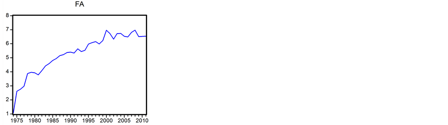

Figure 1. Series are non-stationary at level. Source: Economic survey, Various issues, Ministry of finance, Government of Nepal.


Figure 2. Series become stationary at first difference. Source: Economic Survey, Various issues, Ministry of finance, Government of Nepal.
5.4. Unit Root Test
The finding of the ADF test exhibits that all the series under consideration are non-stationary in their level. However, stationarity is found after first deference. The appropriate lag order is 3 selected by using Akaike criteria. The ADF test results are given in Table 1.
5.5. Co-Integration Test
Table 2 represents the Johansen co-integration test results. This table shows whether there is any long-run co-movement between the series under consideration. Test results shows that there are three co-integrating equations indicating a long-run relationship between variables (EC, FA and GDP).
5.6. OLS Estimation Results at Level
The co-integration test suggests that a regression equation can be set up between electricity consumption and explanatory variables in levels. OLS estimation is more important to detect the spurious regression. The results of this estimation are given in Table 3.
Table 3 represents results from the ordinary least square estimation of the relationship between EC, FA and GDP. F-statistic (600.3 with probability 0) shows that over all estimation is significant at 1% level and has a strong explanatory power (R-squared is 0.97). Individual coefficients are also significant at 1% level as indicated by t-statistic. It appears from these results that electricity consumption and foreign aid are positively correlated over the time period of 1974-2011. Similar is the case of electricity consumption and gross domestic product. The growth elasticity of foreign aid and GDP in that time period is 0.27 and 2.22 respectively. It indicates that the 1% change in foreign aid and GDP will change the electricity consumption by 0.27% and 2.27% respectively. The elasticity coefficient of FA is less than 1 indicating a less proportional change in electricity demand associated with the change in FA. However, the elasticity coefficient of GDP is greater than 1 indicating a more than proportional change in electricity demand associated with the change in GDP. It implies that change in electricity consumption is more sensitive associated with the change in GDP than the corresponding change in FA.

Table 1. ADF test (unit root test).
*Significant at 1% level; Source: Economic Survey, Various issues, Ministry of finance, Government of Nepal.
Table 2. Results of co-integration test.
*Indicates rejection of hypothesis at 5% level Both trace and Max-eigenvalue test indicates 3 co-integrating eqn(s) at the 0.05 level; Series: EC, FA, GDP; Source: Economic Survey, Various issues, Ministry of finance, Government of Nepal.
Table 3. Results of OLS parameter estimation at level.
*Significance at 1% level. Source: Economic Survey, Various issues, Ministry of finance, Government of Nepal.
Another main purpose of OLS estimation in level is to detect the spurious regression. The estimated result does not show any evidence for this. Durbin-Watson statistics is greater than R-squared. This is the fundamental criteria for having non-spurious regression. Non-spurious regression is the prerequisite to evaluate shortand long-run equilibrium using error correction model (ECM).
5.7. Error Correction Model (ECM)
Co-integration and non-spurious regression are the fundamental requirements of ECM. Results of co-integration test (Table 2) and OLS estimation (Table 3) at level have fulfilled these two conditions. EC, FA and GDP are co-integrated and non-spurious regression. They provide basis to run the ECM on the proposed variables. Shortand long-run equilibrium between the variable EC, FA and GDP in the system have been investigated with the help of ECM as given below.
d(EC) = b3 d(FA) + b4 d(GDP) + b5 Ut − 1 + V d(EC) = first difference of electricity consumption d(FA) = first difference of foreign aid d(GDP) = first difference of gross domestic product Ut-1 = One period lag of residual obtained from the OLS estimation at level b3, b4 and b5 are parameters to be estimated V = Error term Parameters b3 and b4 irrespective of their sign but should be individually significant represent short-run equilibrium between EC, FA and GDP. However, parameter b5 represents long-run equilibrium between the same variable. The sign of b5 should be negative and significant as well for holding long-run equilibrium. Table 4 represents the results of ECM.
The ECM is no spurious regression model as indicated by the R-squared and Durbin-Watson statistics. The coefficient b3 and b4 are positive indicating there is positive relationship between d(EC), d(FA) and d(GDP). b3 is significant at 10% level of significance while b4 at 1%. These are known as the short-run equilibrium coefficients. The coefficient b5 is long-run equilibrium coefficient which also is known as the error correction coefficient. It is negative and significant as desired. The values of these parameters are given in Table 5 to show the shortand long-run equilibrium of the variables under consideration which is the main theme of this investigation.
Table 4. Results of OLS parameter estimation in first difference.
* and ** indicate significant at 1% and 10% level. Source: Economic Survey, Various issues, Ministry of finance, Government of Nepal.
Table 5. Shortand long-run equilibrium.
Source: Based on Table 4.
5.8. The Short-Run Equilibrium
The values of b3 and b4 are 0.08 and 2.31 respectively (Table 5) and they are individually significant at10% and 1% level respectively (see Table 4). These coefficients are known as the short-run coefficients and represent the short-run equilibrium. They tell about the rate at which the previous period disequilibrium of the system is being corrected. The values of b3 and b4 are 0.08 and 2.31 respectively meaning that system corrects its previous period disequilibrium at a speed of 8% between variables EC and FA and 231% between variables EC and GDP.
5.9. The Long-Run Equilibrium
Ut − 1 is one period lag error correction term or residual. It guides the variables (EC, FA and GDP) of the system to restore back to equilibrium or it corrects disequilibrium. To happen this the sign of this should be negative and significant. Parameter b5 represents its coefficient. It tells about the rate at which it corrects the previous period disequilibrium of the system if it is negative and significant. The coefficient of b5 is negative (−0.72, Table 5) and is significant at 1% level (Table 4) meaning that system corrects its previous period disequilibrium at a speed of 72% annually.
6. Summary
This paper examines the relationship between electricity consumption with two explanatory variables-foreign aid and GDP. Electricity consumption is positively associated with foreign aid and GDP. The data of these variables are non-stationary at their level but become stationary at first difference. These series are co-integrated showing the long-run relationship between the variables under consideration. The regression equation is not spurious in its level. It fulfills the prerequisite to apply error correction model to find out the short and long rum equilibrium. Results are robust for analyzing short and long-run equilibrium as indicated by their test statistics.
7. Conclusion
A strong relationship exists between electricity consumption, foreign aid and gross domestic product over the period of 1974-2011. The regression model is not spurious as tested. The time series data of these variables contain unit root and they become stationary after conducting ADF test. They have long-run relation as indicated by Johansen co-integration test. The statistically significant elasticity coefficient of OLS estimation at some level expresses that the 1% change in foreign aid and GDP will change the electricity consumption by 0.27% and 2.27% respectively. The results of ECM indicate that there are both shortand long-run equilibriums in the system. The coefficient of one period lag residual coefficient is negative and significant which represents the long-run equilibrium. The coefficient is −0.72 meaning that system corrects its previous period disequilibrium at a speed of 72% annually.