Open Journal of Modern Hydrology
Vol.3 No.3(2013), Article ID:34064,16 pages DOI:10.4236/ojmh.2013.33018
Combined Effect of Infiltration, Capillary Barrier and Sloping Layered Soil on Flow and Solute Transfer in a Heterogeneous Lysimeter
![]()
Laboratoire d’Ecologie des Hydrosystèmes Naturels et Anthropisés, UMR 5023 CNRS-ENTPE-UCBL, Université de Lyon, Lyon, France.
Email: *angulo@entpe.fr
Copyright © 2013 Le Binh Bien et al. This is an open access article distributed under the Creative Commons Attribution License, which permits unrestricted use, distribution, and reproduction in any medium, provided the original work is properly cited.
Received March 26th, 2013; revised April 27th, 2013; accepted May 5th, 2013
Keywords: Capillary Barrier; Lysimeter; Preferential Flow; Unsaturated Soil
ABSTRACT
This aim of this paper is to describe a study of the combined effect of infiltration, capillary barrier and sloping layered soil on both flow and solute transport processes in a large, physical model (1 × 1 × 1.6 m3) called LUGH (Lysimeter for Urban Groundwater Hydrology) and a 3D numerical flow model. Sand and a soil composed of a bimodal sand-gravel mixture were placed in the lysimeter to simulate one of the basic structural and textural elements of the heterogeneity observed in the vadose zone under an infiltration basin of Lyon (France). Water and an inert tracer (KBr) were injected from the top of the lysimeter using a specific water sprinkler system and collected at 15 different outlets at the bottom. The outlet flows and the 15 breakthrough curves obtained presented high heterogeneity, emphasising the establishment of preferential flows resulting from both capillary barrier and soil layer dip effects. Numerical modelling led to better understanding of the mechanisms responsible for these heterogeneous transfers and it was also used to perform a sensitivity analysis of the effects of water velocity (water and solute flux fed by the sprinkler) and the slope interface. The results show that decreasing velocity and increasing the slope of the interface can lead to the development of preferential flows. In addition, the offset of the centre of gravity of the flow distribution at the output increases linearly as a function of the slope angle of the layered soil. This paper provides relevant information on the coupling between hydrodynamic processes and pollutant transfer in unsaturated heterogeneous soil and emphasizes the role of the geometry of the interfaces between materials and boundary conditions as key factors for preferential flow.
1. Introduction
Stormwater runoff is loaded with different contaminants (heavy metals, pesticides, fertilisers, etc.) of agricultural origin [1] and urban origin [2]. Consequently, when infiltrating the soil, the runoff water loaded with significant quantities of contaminants reaches the vadose zone and migrates to the groundwater [3] representing a major environmental issue.
The vadose zone plays a predominant role in the transfer of water and solutes as it occupies a central position for exchanges and interactions with the other compartments (atmosphere, biosphere, groundwater, etc.). The question raised is always that of how the contaminants that spread on the surface of the soil are transferred to this zone, and when, where and in what proportion they reach the groundwater. Many authors have emphasized that this process is closely associated with preferential flows that participate in accelerating the transfer to the groundwater [4]. The evolution of these preferential flows depend on the heterogeneity of the texture [5-7] and the structure [8-10] of the soil and the soil moisture regime (i.e. moisture history, intensity and volume of precipitations) [11,12].
Many studies focused on coupled water-solute transfers have been carried out in the vadose zone by in-situ tracing [13-15]. Field tests have the advantage of being carried out under real conditions and highlight the influence of the vadose zone on the transfer of the solutes. However, the interpretation of results remains difficult given the myriad non controlled parameters involved: initial and boundary conditions, the geochemical quality of the water and materials, and the spatial variability of the lithology and structure of the vadose zone.
One of the alternatives to field tests is to perform laboratory studies using leaching columns. This technique, although accurate regarding the identification of certain transfer mechanisms [16-19], allows estimating the key parameters of water flow and the transport of solutes in unsaturated soils according to one dimensional geometry only. Since leaching columns are one-dimensional devices, their results are difficult to use for studying preferential flows in the field with two and three dimensional geometry.
Consequently, laboratory 3D pilot devices have been developed to study preferential flows under controlled conditions. Metric scale laboratory lysimeters are widely used [20] to better understand the water and solute transfer process in porous media [11,12,21,22]. They provide an intermediate approach between the two scales, i.e. the laboratory leaching column and a plot of land used for field studies. In these studies, no attempt was made to determine the effect of heterogeneity on coupled water and solute transfer mechanisms in an unsaturated medium. Abdou and Flury [23] focused on the role of heterogeneous structures and the impact of scale between a lysimeter and a test in the field. Nonetheless, their studies only dealt with numerical works performed in two dimensions. In all the studies mentioned above, the lysimeters were supplied with water uniformly over the entire surface of the soil. Thus the water tended to flow vertically while lateral flows were limited.
In this article, we present a methodology designed to improve and validate a conceptual and numerical model of the hydrodynamics in heterogeneous soil using a laboratory pilot rig. The purpose of this rig, known as LUGH (Lysimeter for Urban Groundwater Hydrology) [24], is to provide a 3D representation of the structural and textural heterogeneities observed in the fluvioglacial formations in the east Lyon region (France). This model permits studying in particular the initial and boundary conditions imposed and their role in preferential flows. The LUGH lysimeter is supplied only on one part of its surface to permit lateral flows, free drainage and the collection of the effluents distributed at several different outlets. This subdivision of effluents provides an extended view of the spatial and temporal distribution of solutes at the outlet of the lysimeter. The comparison of the numerical and experimental data makes it possible to test and validate transfer models coupling different processes in 3D and thus take into account the effect of the medium’s heterogeneity and the effect of the boundary condition at the bottom of the lysimeter. The numerical resolution of different scenarios then permits testing the influence of infiltration speed and the slope at the interface between two different materials on the establishment of heterogeneous flows.
2. Materials and Methods
2.1. Water Flow and Solute Transport
Modelling the transfer of water and solutes is based on the Darcy approach. Darcy’s 3D flow is assumed to occur in the unsaturated porous medium studied with the LUGH lysimeter. This flow is characterised by the Richards equation [25] in the following way:
 (1)
(1)
where the capillary capacity, C(h) [L−1], is the variation of the volumetric water content q [L3L−3] b pressure head h [L], H [L] is the hydraulic head and K(q) [LT−1] is the unsaturated hydraulic conductivity, which depends on q or h, and Ñ refers to the Nabla operator.
The functions of the usual water retention curve q (h) and the hydraulic conductivity K(h) to describe the flows in the unsaturated zone are given by van Genuchten equations with the Mualem condition [26,27] :
 (2)
(2)
with α (m–1), m and n being parameters such that m = 1 – 1/n.
 (3)
(3)
with Se [-] being the effective saturation:
 (4)
(4)
where qr [L3L−3] and qs [L3L−3] denote the residual and saturated water contents, Ks [LT−1] is the saturated hydraulic conductivity, l [-] is the connection coefficient of the pores estimated by Mualem [27] at an average of 0.5.
The transport of the non-reactive solute in the porous medium can be modelled by the convection-dispersion equation in an initial approach [28]:
 (5)
(5)
where C [ML−3] is the concentration of the solute in the liquid, D [L2T−1] is the hydrodynamic dispersion coefficient.
D groups the molecular diffusion Do and the kinematic dispersion: 
where Do [L2T−1] is the molecular dispersion, l [L] is the dispersivity, tL [-] is the tortuosity, v [LT−1] is the pore velocity, v = q/θ.
These characteristics are assumed to be homogenous and invariant with humidity. The molecular diffusion Do was obtained from the literature. The longitudinal dispersivity, α1, was preselected according to the maximum grain size of the material as the initial value. Then, all the longitudinal α1 and lateral dispersivities α2 and α3 were optimised by fitting experimental data. In steady state flow, the tortuosity τL was calculated using the volumetric water content as follows [29]:
 (6)
(6)
2.2. Materials
We used fine sand (0 to 2 mm in diameter) and gravel (4 to 10 mm in diameter). A third bimodal material was a mixture composed of sand and gravel, each making up 50% in weight. This proportion was chosen to ensure the bimodal grain size distribution of the third material. The grain sizes of the three materials were similar to those observed on the most common litho-facies found in the east Lyon region [30]. The hydrodynamic characteristics of the sand and the bimodal material were estimated individually using the BEST method [31], validated analytically [32,33] and experimentally to characterise the comparable matrices resulting from the fluvioglacial deposits of the east Lyon region [34] and those of other types of coarse material [7,35,36]. Then the hydrodynamic characteristics obtained were optimised using the RETC software [37] to adapt them to Equations (2) and (3) by the method proposed by Mubarak et al. [38]. The results are given in Table 1. The properties of the gravel are without importance given that only the sand and the bimodal material were used in this study.
The LUGH lysimeter (Figure 1(a)) is composed of a PVC (polyvinyl chloride) tank 1.6 m long, 1 m wide and


Figure 1. The LUGH lysimeter and drainage system (at top) and profiles used with positions of TDR sensors (at bottom).

Table 1. Hydrodynamic and hydrodispersive parameters used for modelling the LUGH lysimeter with COMSOL.
1 m deep. Fifteen concrete blocks (0.32 × 0.32 × 0.15 m3) are arranged at the bottom of the lysimeter (Figures 1(b) and (c)) in the form of a funnel to recover the eluents in the lower boundary conditions. These blocks are labelled in the form of a matrix in 3 lines (A, B, and C) and 5 rows (1 to 5). The walls of the tank and the surface of the concrete blocks are covered by a watertight and nonreactive geomembrane that ensures the system is impermeable. A hole is pierced at the centre of each concrete block to permit free drainage and the collection of the effluent. Six TDR sensors (Time Domain Reflectometry, model CS616, Campbell Scientific, Logan, UT) with two rods 0.3 m long are placed at strategic points of the lysimeter to obtain a profile of the volumetric water content in the soil and next to the interfaces (Figures 1(d) and (e)). They are linked by an automatic acquisition system used to record the measurements every minute during the test.
The water (groundwater with an electric conductivity of 522 μS∙m−1) and the tracer solution were supplied along a strip 0.32 m long placed across the width of the lysimeter by an automatic spraying system (Figure 1(a)). Sprinklers are used to obtain relatively uniform humidification when calibrated at a given height and hydraulic supply pressure. Two solenoid valves upstream of the sprinklers, linked to PLCs, permit pulsed regulation of the discharge. The inlet flow is controlled by a series of closely spaced time windows which, given the time frame of the test, allow considering the supply as continuous. The hydraulic supply circuit is equipped with a three-way valve to permit switching between supplying the water and the tracer solution (stored in a plastic tank).
Two soil profiles were compacted in the LUGH lysimeter (Figures 1(d) and (e)). The first profile (PROF1) was produced only with the bimodal material (ρd = 1794 kg∙m−3). This mixture is analogous to the material found in large proportions in the fluvioglacial deposits of the Django Reinhardt site [30] and is used as a control (homogenous soil). The water and solute supply zone is placed vertical to row 3.
The second profile (PROF2) is composed of a layer of sand (ρd = 1634 kg·m–3) placed above a layer of the bimodal mixture (ρd = 1794 kg·m–3) forming an interface with a slope of 25% (angle of the interface in relation to the horizontal Φ = 14˚). This profile represents the usual case observed in the field of a fine material deposited on a coarse material, implying the development of a capillary barrier [9,10,13,39]. In this case, the supply zone is slightly off-centre to the right, vertical to rows 3 and 4, to highlight the capillary barrier effect on the part downstream of the supply zone.
2.3. Protocols of the Infiltration test and Flow Tracing
Two experimental tests performed on the two profiles PROF1 and PROF2 are called E1 and E2 respectively. In each test, the lysimeter is sprayed at Darcian velocity q1= 3.62e−5 ms−1 until the establishment of a steady state flow (i.e. constant flow at the outlet, and measurements of constant water content). Then, by switching the supply, a solution of potassium bromide (KBr) at a concentration of 10−2 moll−1 is supplied by pulse injection. The total volume of the solute supplied is 0.03 m3 corresponding to a half pore volume, Vp, of the material placed directly under the infiltration zone, i.e.:
 (7)
(7)
where Sinf [L2] is the surface area of the infiltration, Sinf = 0.96 × 0.32 m2, eZNS [L] is the total thickness of the profile, eZNS = 0.6 m, ε [-] is the total porosity, ε = 0.329 for PROF1 and ε = 0.353 for PROF2, i.e. 0.0606 m3 and 0.0651 m3 for PROF1 and PROF2, respectively.
Once the tracer pulse has been applied, the lysimeter continues to be supplied with water to “wash the system” and recover the tracer at the outlet, while keeping the Darcy velocity constant (steady state flow).
The quantity of water at the outlet of the 15 sampling blocks is recorded through time to characterise the flow rates leaving the system. For each outlet, we define wi, the ratio between the volume of water eluted locally and the total volume injected to quantify the water balance. Then, the concentrations in bromide are determined by electric conductimetry (electric conductimeter LF 318/ SET) and ionic chromatography (DIONEX DX-100 Ion Chromatograph).
The elutions at the outlet of the 15 sampling blocks are processed classically by a dynamic systems approach by considering the flows of water measured at the outlet. The inlet signal is a pulse of solute at concentration C0 and duration dt. The moments of order N are calculated at the outlet according to the following expression:
 (8)
(8)
For each elution curve, we calculate the mass balance, the mean residence time and the variance.
The mass balance of the solute, MB [-], of each outlet is calculated from the moment of order 0 and from the quantity injected at the inlet [40]:
 (9)
(9)
A global mass balance is also calculated at the scale of the lysimeter, by the following relation to verify the conservative character of the tracer:
 (10)
(10)
where wi is the proportion of the discharge at the outlet.
The average residence time of the solute corresponds to the difference between the mean time of the breakthrough of the solute at the outlet minus the mean time of the entry of the solute at the inlet. This is calculated on the basis of the moment of order 1 and the moment of order 0 by [40]:
 (11)
(11)
The variance is calculated with the moment of order 2; it permits evaluating the degree of spread of the elution curves:
 (12)
(12)
2.4. Numerical Modelling
Equations (1) and (5) are solved using calculation codes implemented in COMSOL Multiphysics [41]. The flow domain is divided into a tetrahedral mesh. It is tighter around the supply zone, at the base of the lysimeter and at the interface between the two materials for profile PROF2. In our study, the flow domains are discretized by 29,300 elements for profile PROF1 and by 37,100 elements for profile PROF2, respectively. The highest number of cells for the second case results from finer meshing next to the interface between the two materials. The lower boundary condition represents the outlet of the effluents through squares measuring 0.1 × 0.1 m2. These squares correspond to the area of the filtering layer placed at the bottom of each concrete block of the lysimeter. The lower boundary condition corresponds to a free drainage condition (unit hydraulic gradient) giving rise to the following expression for the outlet velocity:
 (13)
(13)
where [LT−1] is the Darcian velocity of the effluent in each outlet, Ks [LT−1] is the saturated hydraulic conductivity, kr [-] is the relative permeability taking into account the partial saturation of the material.
The negative sign indicates a flow leaving the lysimeter. The upper supply zone is represented by a uniform flow condition, whereas the rest of the surfaces correspond to a null flux boundary condition.
The experimental data of tests E1 and E2 are used to validate the 3D numerical model as well as the choice of the hydrodynamic and hydrodispersive parameters of the materials. Once the model had been validated, a sensitivity test (25 different flow scenarios) based on the geometric configuration of test E2 (heterogeneous profile) was performed to quantify the impact of the supply velocity (5 different velocities) and the slope angle (5 different angles) on the transfer of the water and the solute in the lysimeter (Table 2). The supply zone in the sensitivity test was placed astride rows 3 and 4, as in the case of test E2. Moreover, the vertical distance from the cen tre of the supply surface until the interface between the two materials was fixed at z = 0.34 m as in test E2. These velocities guaranteed the flows in the domain of validity of the Darcy equation and corresponded to the velocities used classically for studies of solute transfer in lysimeters [11,12,22]. They ensured the different and contrasted unsaturated moisture conditions of the lysimeter susceptible to influence capillary barrier phenomena.
3. Results and Discussion
3.1. Offset of Centre of Gravity of Outlet Flows
Under the uniform profile condition, the distribution of outlet flows in steady state of test E1 was almost symmetrical. There was a negligible diversion of the centre of gravity of the volume of infiltrated water, and of the centres of gravity at the corresponding outlet and inlet (Figure 2(a)). Below the supply zone (at the vertical of row 3), the discharges at the outlet of row 3 were higher and reached 30% of the total (sum of discharges of outlets A, B, and C). However, the discharges at the outlet

Figure 2. Top: relative discharge in steady state at each outlet (curves) and mean in each row (bars). Bottom: measured (dotted lines) and simulated (lines) elution curves; each curve corresponds to the mean of each row.

Table 2. Infiltration velocity at the surface and the slope angle of the sensitivity test.
of the lateral rows of the lysimeter (rows 1 and 5) also reached quite high values. The sum of the relative discharges of outlets 1A, 1B, and 1C was 14%, and that of outlets 5A, 5B and 5C was 11%. This shows that a large quantity of water flowed laterally. The TDR sensors indicated the possible existence of a zone in which water accumulated at the bottom of the lysimeter. It was also noted that these lateral flows were perfectly symmetrical: the sum of the discharges from rows 1 and 2 was equal to the sum of the discharges from rows 4 and 5.
Conversely, the distribution of the effluents of test E2 (supply zone centred on the vertical of rows 3 and 4) shows a large shift between the centres of gravity of the water at the outlet and the inlet (Figure 2(c)). The position of the latter was diverted by 13.5 cm downstream of the slope in comparison to that of the inlet. 62.3% of the discharge exited downstream (rows 1, 2, and 3) and the rest, 37.7%, exited upstream (rows 4 and 5). Furthermore, the results of the TDR sensors showed that water accumulated in the sand along the interface between the two materials (Figure 3). Part of the flux of water arriving at the interface between the two materials therefore seems to have been diverted along the slope, simultaneously producing an increase in water content at the interface, a shift of the centre of gravity downstream and the uniformisation of the discharges of rows 2, 3, and 4. It was assumed that these preferential flows resulted from the effect of the capillary barrier at the interface between the two materials.
3.2. Elution Curves
The shapes of the bromide elution curves of the central rows (rows 2, 3, and 4) of test E1 (Figure 2(b)) were similar with peaks of the same order of magnitude, around the value C/C0 = 0.7. Their tails decreased rapidly and almost simultaneously during the leaching phase

Figure 3. Distribution of volumetric water content, stream lines and vector field (a), (b); insert: comparison of the simulated (curves) and measured (dotted lines) water content. Bottom: transfer of solute as a function of time; t = 0.75 h corresponds to the moment of stopping the solute injection (c)-(h).
following the solute pulse. On the contrary, the solute appeared later in rows 1 and 5; the elution curves of these two rows were more spread out with lower peaks. The difference between the elution curves was representative of the spatial distribution of the solute at the bottom of the LUGH lysimeter. The solute arrived earlier at the centre and at higher concentrations, and then spread symmetrically on both sides.
At the scale of the lysimeter, the mass balance of the system was close to 1. Likewise, the mass balances were close to 1 for almost all the outlets (Table 3). We recorded values slightly lower than 1 for rows 1 and 5, showing incomplete elution linked to an insufficiently long experiment time (Figure 2(b)). The mass balance values demonstrated the conservative nature of the tracer, which followed the water perfectly.

Table 3. Characteristic parameters of the elution curves of tests E1 and E2; each value is the mean of lines A, B, and C of the same row (1 to 5).
The residence times and standard deviations of rows 2, 3, and 4 were of the same order of magnitude. In combination with the distribution of discharges (Figure 2(b)), the flow zone formed by rows 2, 3, and 4 played a dominant role in solute transfer: up to 75% of the solute passed by these three rows, corresponding perfectly to the fraction of water eluted by them. Indeed, the solute transferred mostly vertically, following paths with short distances. Conversely, the residence times, variances and standard deviations of the elution curves of rows 1 and 5 were higher, thus indicating longer solute flow paths to these two outlets. This transfer characteristic resulted from the lateral flows induced by edge effects.
The elution curves of test E2 (Figure 2(d)) are also divided into two groups: the curves of the central rows (rows 2, 3, and 4) with high peaks and short tails and the curves of the sides (rows 1 and 5) that have low peaks and lags as well as very long tails. Analysis of the elution curves highlighted the diversion of the flow linked to the interface. Without the effect or diversion, the flow would have been perfectly symmetrical in comparison to the barycentre of the inlet positioned between rows 3 and 4. In this case, the elutions of rows 3 and 4 would have been the same. Likewise, the elutions of rows 2 and 5 would have been superposed. On the contrary, the data show that this was not the case. The solute transfer of row 3 was the fastest whereas the solute transfers of rows 1 and 2 were comparable to those of rows 5 and 4 respectively. These trends can be explained by a diversion of fluxes along the slope responsible for the shift of the solute downstream of the slope. Furthermore, the transfer of the solute in test E2 lasted longer and the elution curves were more spread out than for test E1, indicated by a longer residence time (Table 3).
The mass balance of the solute, calculated between 0 and 10 h for test E2, reached the value of 0.96 (Table 3). The solute injected was therefore recovered well at the outlet, mainly by the rows located at the centre of the lysimeter (rows 2, 3 and 4). The mass balance was slightly underestimated due to the more significant spreading of the elution curves of rows 1 and 5 which had non null concentrations at t = 10 h (Figure 2(d)).
As with test E1, the results between the three series A, B and C were of the same order of magnitude but with larger differences in test E2 (Table 3). These differences were due to the local modification of the flow introduced by the interface between the two materials in test E2. These modifications were not present in test E1 in a homogeneous medium.
3.3. Validation of the Numerical Model
In steady state, the numerical model E1 was first validated by comparing it with the measurements of volumetric water content (TDR sensors). The results (Figure 3(a)) show that the simulated values are quite close to the experimental values. The calculated moisture profile predicted a saturated zone at the bottom of the LUGH lysimeter.
As with test E1, the volumetric water contents modelled for test E2 were compared to the TDR measurements. The difference between the simulated data and the experimental data was slightly larger than in the previous case. Nonetheless, the model and the measurements corresponded when taking the error margin relating to the measurements into account. The reduction of the correspondence between the model and the experiment can be explained by the sensitivity of the TDR sensors. Since the distance between the two rods of the TDR sensor was 5 cm, it can be assumed that the measurement was performed on the volume of influence of the sensor, in the order of 5 to 10 cm in diameter around the rods. Averaging the volume probed did not permit detecting the contrast of volumetric water content at the interface between the two materials, or the existence of a zone of water accumulating in the form of a more or less thick film of water on the sand side. Nonetheless, the results of the TDR sensors of test E2 clearly show the existence of a water accumulation zone at the interface between the two materials: the volumetric water content in the sand is higher than the volumetric water content in the bimodal material along the interface (Figure 3(b)). This increase in water content may stem from capillary retention capacities or to the diversion of flows due to the interface.
The numerical simulation of tests E1 and E2 was performed by assuming the symmetry of initial and boundary conditions through the width of the LUGH. In addition, the results of the simulation of the outlets positioned on series A, B and C are the same. The elution curves simulated on line B were calculated over 10 hours, counting from the application of the tracer. The eluted solute was obtained by integrating the distribution of the calculated concentrations crossing the surface of the squares at the bottom of the lysimeter. The calculated elution curves were then compared for the five rows (rows 1, 2, 3, 4 and 5) with the mean of the experimental elution curves (mean of lines A, B and C, Figures 2(b) and (d)).
In terms of transfer, the results of the model of test E1 represented the same trends as the curves measured on the five rows well (Figure 2(b)). This allowed us to validate coupling the Richards equation with the convection-dispersion equation for the study of water flow and solute transfer in model E1.
The numerical results provided the volumetric water content field and the vector field of the Darcy flux permitting us to study the water and solute transfer process in the LUGH lysimeter. We observed that, in test E1, the vertical flux corresponding to gravity flow mechanisms dominated with high velocities below the supply zone. The trajectory of the flow was almost vertical and the stream lines were diverted only near the bottom of the lysimeter (rows 2 to 4, Figure 3(a)). The fluxes of rows 1 and 5 were weak and dispersed. This explains the clear difference between the elution curves of rows 2 to 4, at the centre, and those of rows 1 and 5, at the sides. Indeed, the lower boundary condition is a condition of free drainage. However, the water is only drained when a layer of soil just above the bottom of the lysimeter reaches saturation [23]. This accumulation zone developed progressively, and at steady flow state, it was larger at the centre of the lysimeter and decreased towards the sides, thereby leading to the diversion of the flows at the bottom of the lysimeter. The presence of this accumulation and the induced lateral flows may have resulted from the finite geometry of the lysimeter and the proximity of the lower boundary condition. A numerical study that varied the dimension of the system tended to show that the lateral flows lessened at the same depth when the boundary condition was lowered (data not illustrated). These lateral flows are responsible for the output of the fluxes of water and solutes in rows 1 and 5 with a lag due to a trajectory longer than that for rows 2 to 4. The model therefore made it possible to demonstrate that the finite geometry of the lysimeter led to lateral flows and explain the outputs observed at the edge of the system (rows 1 and 5). In the field, where water can flow freely at depth, there is no such lower limit and transfers are essentially vertical.
The hydrodynamic and hydrodispersive parameters of the bimodal material were conserved following the optimisation step of model E1 and applied to the water and solute transfer conditions specific to case E2. The results of E2 showed that the outputs upstream of the slope (rows 3, 4 and 5) were simulated well and a little more lag (residence times) for the two outputs downstream (rows 1 and 2). As with the tortuosity parameter, the uncertainty obtained on dispersivities α1, α2, and α3 could be relatively large. Theoretically, an uncertainty on the dispersitivity and tortuosity parameters should affect the dispersion of the elution peak though not its position [40]. This uncertainty is overlapped by that on the other parameters of the model (θr, θs, α, n, and Ks) for the two different materials which may explain the slight differences between the models and the measurements. Nonetheless, in our study, the differences between simulation and observation were considered acceptable and confirmed the model’s capacity to reproduce the hydrodynamic hydrodispersive behaviour of model PROF2 of the LUGH lysimeter.
As with the case of profile PROF1, studying the distribution of volumetric water content and the vector field of the Darcy flux provided valuable information on the water and solute transfer process in the PROF2 system. The distribution of volumetric water content in E2 demonstrated the presence of a capillary barrier which was the cause underlying the accumulation of water at the interface between the two materials (Figure 3(b)). It resulted from the contrast between the hydrodynamic characteristics of these materials. For the same capillary pressure along the interface, the hydraulic conductivity in the sand was always greater than that in the bimodal material. From the hydrological standpoint, the lower layer, in this case bimodal, was less permeable, thus impeding the entire transfer of the flux through the interface, since part of the flux was diverted along it.
When the water arrived at the interface between the two materials, it accumulated in the sand, increasing capillary pressure locally before penetrating the bimodal medium. The form of the accumulation zone on an inclined plane developed progressively upstream and downstream from the supply zone asymmetrically due to gravity and capillarity. Below the interface, the hydrodynamic contrast between the two materials limited the volumetric water content in the bimodal medium and the flow returned to the vertical direction. Moreover, the flow velocity, indicated by the vector field of the flux, was quite low.
The water and the solute were then dispersed and distributed almost throughout the volume of the bimodal zone. The trajectory of the flow from the source (supply) was therefore extended by the effect of the slope and the residence time of the solute increased in comparison to test E1 (Figures 3(c)-(h)). Water accumulated at the bottom of the lysimeter in a similar way to that of test PROF1. However, the effect of the lower boundary condition appeared less pronounced.
Modelling the flow clarified understanding of solute transfers insofar as they followed the same path as the water. As with test E1, in test E2, the solute first passed through the sand symmetrically in relation to the supply surface. Then, the plume of solute was deformed by the capillary barrier and the slope of the interface. At the end of the solute pulse (t = 0.75 h), the quantity of solute present in the sand was pushed by the water (t > 0.75 h). The preferential transfer in the lysimeter was illustrated by the evolution of the shape of the plume corresponding to the zones of strongest concentrations. It is clear that the plume shifted along the interface. The volumes of solute injected and the input velocities of water and solute were the same for E1 and E2. The evolution through time of the relative concentration profile, C/C0, of profile E2 presented a slight lag in comparison to that of profile E1. As a function of time, the horizontal dispersion in E2 was greater and penetration was less deep than in case E1. The upstream/downstream shift also appeared clearly. The elutions modelled at the outlet were characterised by this shift and were fully consistent with the experimental data.
3.4. Apparent Capillary Barrier and Moisture History
In this part, we used the validated model to predict the impact of the interface angle and the imposed velocity under upper boundary conditions on preferential flows and several related metrics (diversion of the barycentre of the leached volume, volume of water in the sand and bimodal gravel (associated with the accumulation at the interface), the vertical and horizontal components of the velocity at the interface). Afterwards, we studied the impacts of preferential flows on transfers in terms of residence time.
One of the most obvious consequences of the capillary barrier effect was the diversion of flows of water and solute at the interface between the two materials. This diversion led to a lateral shift of the centre of gravity at the outlet of the lysimeter in comparison to the inlet. Determining this shift is an important characteristic used to quantify the role of the capillary barrier.
The results of the sensitivity test showed that the shift of the centre of gravity of the water between the inlet and the outlet, ΔD [L], all velocities confounded, depended linearly on the slope of the interface (Figure 4(a)). For each velocity qi, this relation is represented as ΔDi = aiΦi + bi with ai and bi being constants. The adjustment of these relations, indicated by the determination coefficient, R2, is high for all five velocities (R2 > 0.998).
The value of bi [L] corresponds to the diversion for the case of a null slope with velocity qi. This value is equal to 1 to 3 cm due to the bias introduced by the offset position of the supply in relation to boundary conditions of the lysimeter. These values remain negligible in comparison to the shifts caused by the inclination of the interface.

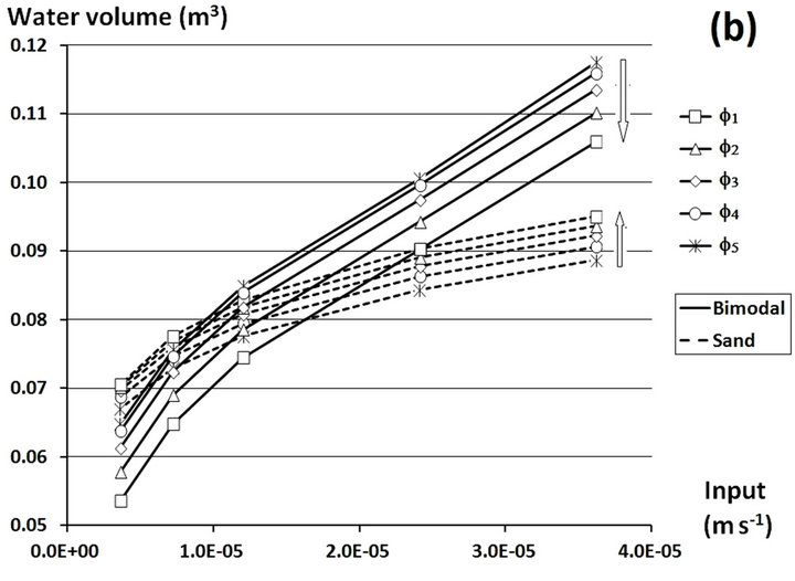
Figure 4. Diversion of the centre of gravity of the water discharges at the outlet as a function of the slope (a) and volume of water in the sand (dotted lines) and in the bimodal medium (lines) as a function of infiltration velocity (b) (the arrows show the trend of increase of angle).
The value of ai [L∙rad−1] corresponding to the tangent of line ΔDi = f(Φi) represents the acceleration of the diversion as a function of the slope. It increases rapidly when the supply velocity decreases. This case shows how the moisture history of the soil and the boundary conditions (represented here by the velocity) can favour the occurrence of a preferential flow. Therefore, at low velocities, the water can flow laterally and preferentially further from the supply zone. The effect of the capillary barrier is more considerable. At a higher velocity, the initial kinetic energy is higher, resulting in significant inertia. The flows therefore deviate less. The value of ai can be calculated using the value of qi as in:
 (14)
(14)
Finally, the diversion of the centre of gravity can be deduced as follows:
 (15)
(15)
This relation permits us to calculate the diversion of the centre of gravity of the water as a function of the infiltration velocity and the slope. This shows that the diversion results from the combined effect of the two factors of slope and imposed velocity at the upper boundary.
The volume of water in the lysimeter is also an important parameter for studying solute transfer. In particular, the presence of the interface results in the accumulation of water in the sand and has an umbrella effect, in turn resulting in a “loss” of water in the underlying gravel. Here, the aim is to link these volumes to the geometry of the system (angle of the interface) and to the boundary conditions.
For the same infiltration velocity, the volume of water contained in the sand increased slightly as a function of the angle of the interface, whereas that in the bimodal material decreased (Figure 4(b)). The variations of the volume of water in the sand and in the bimodal material as a function of the supply velocity were almost the same for the different input velocities. Indeed, curves Ve(Φ) are parallel.
Contrary to the effect of the slope, the velocity affected the stock of water in the lysimeter by favouring the humidification of the overall system. Nonetheless, we observed a more significant change in the bimodal material than in the sand. The variation of the volume of water between the lowest velocity and the highest one in the sand was 33.0% ± 0.91% (average value for the five different slopes), whereas that of the bimodal material was 87.4% ± 5.46%. This difference shows that the accumulation of water at the bottom of the lysimeter (in the bimodal material) was driven more by the increase of the supply velocity than by increasing the angle of the interface. This main characteristic must be taken into account in further studies using lysimeters. Indeed, this accumulation resulting from the lower condition of free drainage also “disturbed” the results.
In order to better understand the water and solute transfer mechanism at the interface between the two materials, the velocity field at the interface was analysed. The aim was to determine how the slope of the interface and the supply velocity acted on components Vy and Vz of the velocity. Component Vx was not counted in this study due to the symmetrical arrangement in the direction of axis x (direction of the length of the lysimeter). The numbering 1 and 2 corresponds to the components in the sand and in the bimodal material respectively.
The values of the horizontal components Vy1 were significantly non null and highlight the horizontal diversion of the flow at the interface (Figure 5). On the contrary, component Vy2, in the bimodal material, was very small. This shows that the part of the water penetrating the interface flowed vertically in the bimodal material. Its lateral diffusion was negligible. When the angle of the interface was null, the horizontal component Vy1 was null at the centre of the injection zone, positive on the right and negative on the left. Thus the flow was diverted to the edges of the lysimeter except at the barycentre of the injection zone (by symmetry) and next to the walls of the lysimeter (tangential flows). The diversion was maximal at about a third of the distance between the barycentre of the injection zone and the sides of the lysimeter. Introducing a slope (relative to the angle) resulted in establishing tangential flows at the interface (directed leftwards) and thus accentuating the corresponding negative values for the horizontal component Vy1. The intersection of the curve of Vy1 with axis y = 0 defines a point of division between the flow upstream and downstream along the slope. This position was strongly dependent on the angle of the interface (Figures 5(a)-(c)). To the left of this point, Vy1 = 0, the water flowed downstream of the slope, and the water running on the interface infiltrated into the underlying layer, explaining why the vertical velocity (and thus the infiltrated flux) was higher, i.e. |Vz1| ≥ |Vz2|. The value of Vy1 and Vz1 in proportion to the value Vz2 increased as a function of the slope (Figures 5(a)-(c)) and decreased as a function of the velocity of infiltration (Figures 5(d)-(f)). This proportion represents the development of preferential flows as a function of the two parameters above.
3.5. Residence Time and the Peaks of Elution Curves of Rows 1 and 3
Rows 1 and 3 were analysed essentially as they are representative of transfers at the centre and at the sides of the lysimeter, respectively. The residence times of row 3 were practically independent of the slope (Figure 6(a)).

Figure 5. Velocity components in the sand (Vy1 and Vz1) and in the bimodal medium (Vy2 and Vz2) as a function of slope and the infiltration velocity.
They depended only on the infiltration velocity. Indeed, the water effluents of row 3 were formed by the fraction of water that penetrated the interface exactly in the direction of the supply. This flux was almost vertical. Likewise, the effect of the slope of the interface on the value of the peak of the elution curve of the solute of row 3 was slight. The effect of the supply velocity in this case is also slight (Figure 6(d)). The values obtained for the relative concentration of the peak of the elution curve of row 3, C/C0, were similar to those of the one-dimensional tests performed in the laboratory column. This can be explained by the transfer mechanism, which was almost one-dimensional close to row 3. The capillary barrier effect in this case is negligible.
Conversely, for row 1, the residence time depended on the slope of the interface and on the inverse of the supply

Figure 6. Comparison of residence time ((a) and (b)); The arrows show the trends of increase of angle and velocity and detail of elution curves for a specific case (c) and the peak of the elution curves of rows 1 and 3 (d).
velocity (Figure 6(b)). In addition, the capillary barrier effect is more obvious for the peak of the solute elution curves. The value of the peak of these curves increases considerably as a function of the slope (Figure 6(d)). This increase stands out more when the supply velocity decreases. This can be explained by the same argument proposed previously to explain the flow field: the fluxes crossing row 1 were generated by the part of the water diverted along the slope. The increase in the diversion of the accumulated water resulted in an increase in the velocity of the water in the direction downstream of the slope. The solute was therefore transferred more rapidly towards row 1. In other words, the preferential flows and their impacts on the solute transfers were favoured when the angle of the interface increased and the supply velocity decreased.
The combined effect of the supply velocity and the slope of the interface on the total elution curve of the lysimeter was also studied (Figure 7). Indeed, this information is often considered to the detriment of more precise sampling. We recall that the total curve was obtained by integrating all 15 elution curves. This curve represents the homogenised behaviour of the lysimeter. The shape of all the total elution curves takes that of a log-normal type of distribution with, however, a tail with a relatively wide spread.
Although the supply velocity was high enough (in this case q1 > q2 > q3), the peak of the total curve was mainly determined by the effluents of the centre of the lysimeter (in particular row 3) which does not depend on the angle of the interface between the two materials. In this case, the curve obtained is slightly dissymmetric and monomodal on which the influence of the angle is weak. The effect of, the angle starts becoming marked from Φ = 10.5˚ for flow rate q4 and at Φ = 7˚ for flow rate q5 (Figure 7(b)). In both the last two cases for which preferential flows were very developed, the elutions of the rows at the sides of the lysimeter (mainly row 1) in creased and contributed more to the total elution. In these cases (smallest velocities), increasing the angle resulted in increasing the dissymmetry of the global curve (Figure 7(d)) with a widening of the tail. This resulted in increasing the contribution of preferential flows at the sides of the lysimeter. We also observed that for each infiltra-

Figure 7. Peak and total volume of water injected as a function of slope and infiltration velocity.
tion velocity, the total volume of water injected necessary to push the solute to the total peak was quite similar, with a slight increase when the slope increased, above all for the lowest velocities. Conversely, this volume decreased and the elution curve was less spread when the velocity decreased. This shows that, for the total curve, the concentration of the solute was higher when velocities were lower.
4. Conclusions
This study focused on the development of a lysimeter for studying the transfer of heterogeneous flows of water and solute in a heterogeneous and unsaturated medium. To do this a pilot LUGH lysimeter was developed and used to observe the flow and transfer of a non-reactive solute in the injection of a steady state flow through the medium. The experimental and numerical results were demonstrated, explaining the occurrence of the capillary barrier phenomenon and the major role played by the initial and boundary conditions of the lysimeter in the establishment of this type of flow.
By using fifteen different outlets, the experimental flow tracing data permitted studying the temporal and spatial evolution of the water discharges and fluxes of solute at the bottom of the lysimeter in comparison to the input at the surface and the configuration of the system. The heterogeneity of the discharges at the outlet, peaks, variances and residence times of the elution curves of these fifteen outlets provided detailed data on the hydraulic behaviour of the heterogeneous system and led to better understanding of the role played by the capillary barrier on the water and solute flows, by taking into account the effect induced by the finite volume of the lysimeter.
The model permitted representing the solute diffusion zone and understanding the effect cause by the presence of the slope between the two materials. Consequently, numerical modelling presents a considerable advantage in explaining the transfer process in the lysimeter. The capillary barrier between two materials in the lysimeter can be quantified by studying the vertical shift between the centres of gravity of the water supply and the distribution of the discharges at the outlet. Under the effect of the capillary barrier in a heterogeneous medium, the water and solute were dispersed, resulting in increased solute residence time in comparison to the homogeneous case.
A series of tests was performed to quantify the impact of supply velocity and slope angle between the two materials on water and solute transfer. It was shown that shift between the centres of gravity of the distribution of the water discharged at the outlet increased linearly as a function of the angle of the interface between the two materials. In addition, reducing the supply velocity and increasing the angle of the interface clearly determined the development of preferential flows. The effect of the bottom of the lysimeter played a very important role in the analysis of the experimental and numerical results. Indeed, the accumulation of water at the base of the lysimeter depended more on the supply velocity than on the capillary barrier effect. Furthermore, the transfer of the solute vertical to the supply zone was practically independent of the angle of the interface. The solute flux at the bottom boundary was impacted by the slope angle mainly for the lowest supply velocity.
From the methodological standpoint, the association of simple tests with a numerical model allowed us to refine the estimation of the key parameters involved in water flow and solute transport. The numerical model permitted both highlighting the behaviour of the coupled water-solute transfer in 3D as a function of space and time and completing the experiments with the sensitivity test in order to pre-dimension new tests.
REFERENCES
- EPA, “Protecting Water Quality from Agricultural Runoff,” US Environmental Protection Agency, 2005.
- EPA, “Protecting Water Quality from Urban Runoff,” US Environmental Protection Agency, 2003.
- J. T. Smullen, A. L. Shallcross and K. A. Cave, “Updating the U.S. Nationwide Urban Runoff Quality Date Base,” Water Science and Technology, Vol. 39, No. 12, 1999, pp. 9-16. doi:10.1016/S0273-1223(99)00312-1
- S. E. Allaire, S. Roulier and A. J. Cessna, “Quantifying Preferential Flow in Soils: A Review of Different Techniques,” Journal of Hydrology, Vol. 378, No. 1-2, 2009, pp. 179-204. doi:10.1016/j.jhydrol.2009.08.013
- J. Bouma, A. Jongerius, O. Boersma, A. Jager and D. Schoonderbeek, “The Function of Different Types of Macropores during Saturated Flow through Four Swelling Soil Horizons,” Soil Science Society of America Journal, Vol. 41, No. 5, 1977, pp. 945-950. doi:10.2136/sssaj1977.03615995004100050028x
- K. J. Beven and P. Germann, “Macropores and Water Flow in Soils,” Water Resources Research, Vol. 18, No. 5, 1982, pp. 1311-1325.
- P. Cannavo, L. Vidal-Beaudet, B. Bechet, L. Lassabatère and S. Charpentier, “Spatial Distribution of Sediments and Transfer Properties in Soils in a Stormwater Infiltration Basin,” Journal of Soils and Sediments, Vol. 10, No. 8, 2010, pp. 1499-1509. doi:10.1007/s11368-010-0258-7
- D. E. Hill and J.-Y. Parlange, “Wetting Front Instability in Layered Soils,” Proceedings of the Soil Science Society of America, Vol. 36, No. 5, 1972, pp. 697-702.
- T. Miyazaki, “Water Flow in Unsaturated Soil Layered Slopes,” Journal of Hydrology, Vol. 102, No. 1-4, 1988, pp. 201-214. doi:10.1016/0022-1694(88)90098-4
- K.-J. S. Kung, “Preferential Flow in a Vadose Zone: 2. Mechanism and Implications,” Geoderma, Vol. 46, No. 1-3, 1990, pp. 59-71. doi:10.1016/0016-7061(90)90007-V
- M. T. Walter, et al., “Funneled Flow Mechanisms in a Sloping Layered Soil: Laboratory Investigation,” Water Resources Research, Vol. 36, No. 4, 2000, pp. 841-849.
- B. Bussière, S. A. Apithy, M. Aubertin and R. P. Chapuis, “Water Diversion Capacity of Inclined Capillary Barriers,” Proceedings of the 56th CGS-IAH Conference, Winnipeg, 29 September-1 October 2003, pp. 192-200.
- A. Heilig, T. S. Steenhuis, M. T. Walter and S. J. Herbert, “Funneled Flow Mechanisms in Layered Soil: Field Investigations,” Journal of Hydrology, Vol. 279, No. 1-4, 2003, pp. 210-223. doi:10.1016/S0022-1694(03)00179-3
- S. Kaskassian, et al., “L’essai d’Infiltration Couplé à un Traçage Non-Réactif: Un Outil Pour Evaluer le Transfert des Polluants dans la Zone Non-Saturée des Sols,” L’eau, l’Industrie, les Nuisances, Vol. 349, 2012, pp. 38-45.
- K.-J. S. Kung, “Preferential Flow in a Sandy Vadose Zone: 1. Field Observation,” Geoderma, Vol. 46, 1990, pp. 51-58.
- L. Février, “Transfert d’un Mélange Zn-Cd-Pb dans un Dépôt Fluvio-Glaciaire Carbonate. Approche en Colonnes de Laboratoire,” Ph.D. Thesis, Ecole Nationale des Travaux Publics de l’Etat, Lyon, 2001.
- L. Lassabatère, T. Winiarski and R. Galvez Cloutier, “Retention of Three Heavy Metals (Zn, Pb and Cd) in a Calcareous Soil Controlled by the Modification of Flow with Geotextiles,” Environmental Science and Technology, Vol. 38, No. 15, 2004, pp. 4215-4221. doi:10.1021/es035029s
- E. Lamy, L. Lassabatère, B. Bechet and H. Andrieu, “Modeling the Influence of an Artificial Macropore in Sandy Columns on Flow and Solute Transfer,” Journal of Hydrology, Vol. 376, No. 3-4, 2009, pp. 392-402. doi:10.1016/j.jhydrol.2009.07.048
- L. Lassabatère, et al., “Concomitant Zn-Cd and Pb Retention in a Carbonated Fluvio-Glacial Deposit under Both Static and Dynamic Conditions,” Chemosphere, Vol. 69, No. 9, 2007, pp. 1499-1508. doi:10.1016/j.chemosphere.2007.04.053
- C. Lanthaler, “Lysimeter Stations and Soil Hydrology Measuring Sites in Europe—Purpose, Equipment, Research Results, Future Developments,” A Diploma Thesis for the Degree of Magistra der Naturwissenschaften, School of Natural Sciences, Karl-Franzens-University, Graz, 2004.
- R. Schoen, J. P. Gaudet and T. Bariac, “Preferential Flow and Solute Transport in a Large Lysimeter, under Controlled Boundary Conditions,” Journal of Hydrology, Vol. 215, No. 1-4, 1999, pp. 70-81. doi:10.1016/S0022-1694(98)00262-5
- T. P. Anguela, “Etude du Transfert d’Eau et de Solutés dans un sol à Nappe Superficielle Drainée Artificiellement,” Ph.D. Thesis, Ecole Nationale du Génie Rural, des Eaux et Forêts, Paris, 2004.
- H. M. Abdou and M. Flury, “Simulation of Water Flow and Solute Transport in Free-Drainage Lysimeters and Field Soils with Heterogeneous Structures,” European Journal of Soil Science, Vol. 55, No. 2, 2004, pp. 229-241.
- L. B. Bien, X. Peyrard, L. Lassabatère, T. Winiarski and R. Angulo-Jaramillo, “Transferts d’Eau et de Particules dans la Zone Non-Saturée Hétérogène: Développement du Pilote de Laboratoire LUGH,” Proceedings of the 35 Ième Journées du GFHN, Louvain-la-Neuve, Belgique, 23-25 Novembre 2010, pp. 165-168.
- L. A. Richards, “Capillary Conduction of Liquids through Porous Mediums,” Physics, Vol. 1, No. 5, 1931, pp. 318- 333. doi:10.1063/1.1745010
- M. T. van Genuchten, “A Closed form Equation for Predicting the Hydraulic Conductivity of Unsaturated Soils,” Soil Science Society of America Journal, Vol. 44, No. 5, 1980, pp. 892-898. doi:10.2136/sssaj1980.03615995004400050002x
- Y. Mualem, “A New Model for Predicting the Hydraulic Conductivity of Unsaturated Porous Media,” Water Resources Research, Vol. 12, No. 3, 1976, pp. 513-522. doi:10.1029/WR012i003p00513
- J. Bear, “Dynamics of Fluids in Porous Media,” American Elsevier, New York, 1972, p. 764.
- R. J. Millington and J. P. Quirk, “Permeability of Porous Media,” Transactions of the Faraday Society, Vol. 57, 1961, pp. 1200-1207. doi:10.1039/tf9615701200
- D. Goutaland, et al., “Hydrostratigraphic Characterization of Glaciofluvial Deposits Underlying an Infiltration Basin Using Ground Penetrating Radar,” Vadose Zone Journal, Vol. 7, No. 1, 2008, pp. 194-207. doi:10.2136/vzj2007.0003
- L. Lassabatère, et al., “Beerkan Estimation of Soil Transfer Parameters through Infiltration Experiments—BEST,” Soil Science Society of America Journal, Vol. 70, 2006, pp. 521-532. doi:10.2136/sssaj2005.0026
- L. Lassabatère, R. Angulo-Jaramillo, J. M. Soria Ugalde, J. Simunek and R. Haverkamp, “Analytical and Numerical Modeling of Water Infiltration Experiments,” Water Resources Research, Vol. 45, 2009, Article ID: W12415.
- P. Nasta, L. Lassabatère, M. Kandelous, J. Simunek and R. Angulo-Jaramillo, “Analysis of the Role of Tortuosity and Infiltration Constants in the Beerkan Method,” Soil Science Society of America Journal, Vol. 76, No. 6, 2012, pp. 1999-2005. doi:10.2136/sssaj2012.0117n
- L. Lassabatère, et al., “Effect of the Settlement of Sediments on Water Infiltration in Two Urban Infiltration Basins,” Geoderma, Vol. 156, No. 3-4, 2010, pp. 316-325. doi:10.1016/j.geoderma.2010.02.031
- E. Gonzalez-Sosa, et al., “Impact of Land Use on the Hydraulic Properties of the Topsoil in a Small French Catchment,” Hydrological Processes, Vol. 24, No. 17, 2010, pp. 2382-2399.
- D. Yilmaz, L. Lassabatère, R. Angulo-Jaramillo and M. Legret, “Hydrodynamic Characterization of Basic Oxygen Furnace Slags through Adapted BEST Method,” Vadoze Zone Journal, Vol. 9, No. 1, 2010, pp. 107-116. doi:10.2136/vzj2009.0039
- M. T. Van Genuchten, F. J. Leij and S. R. Yates, “The RETC Code for Quantifying the Hydraulic Functions of Unsaturated Soils,” US Environmental Protection Agency, Oklahoma, 1991.
- I. Mubarak, J. C. Mailhol, R. Angulo-Jaramillo, S. Bouarfa and P. Ruelle, “Effect of Temporal Variability in Soil Hydraulic Properties on Simulated Water Transfer under High-Frequency Drip Irrigation,” Agricultural Water Management, Vol. 96, No. 11, 2009, pp. 1547-1559. doi:10.1016/j.agwat.2009.06.011
- L. B. Bien, R. Angulo-Jaramillo, D. Predelus, L. Lassabatère and T. Winiarski, “Preferential Flow and Mass Transport Modeling in a Heterogeneous Unsaturated Soil,” Proceedings of the First Pan-American Conference on Unsaturated Soils (Pam-Am UNSAT 2013), Cartagena de Indias, 20 - 22 February 2013, pp. 211-216.
- D. Schweich and M. Sardin, “Les Mécanismes D’interation Solide-Liquide et Leur Modélisation: Applications aux Etudes de Migration en Milieu Aqueux,” 1986, pp. 59-107.
- COMSOL AB, “COMSOL Multiphysics User’s Guide, Version 3.5a,” COMSOL AB, Grenoble, 2008, p. 624.
NOTES
*Corresponding author.