International Journal of Geosciences, 2010, 1, 58-65
doi:10.4236/ijg.2010.12008 Published Online August 2010 (http://www.SciRP.org/journal/ijg)
Estimation of the Degree of Saturation of Shallow Soils
from Satellite Observations to Model Soil Slips Occurred in
Emilia Romagna Region of Northern Italy
Lorella Montrasio1, Roberto Valentino1*, Chiara Quintavalla1
1Department of Civil, Environmental, Territory Engineering and Architecture, University of Parma, Parma, Italy
Received June 23, 2010; revised July 12, 2010; accepted August 2, 2010
Abstract
For the development of alert systems for soil slip occurrence, it is important to evaluate the degree of satura-
tion of shallow soils (Sr) over wide areas. Taking into account the possibility to estimate spatial and temporal
variation of soil moisture using remote sensing techniques, a possible correlation between Sr and the daily
output of a sequential data assimilation system called ACHAB (Assimilation Code for HeAt and moisture
Balance) has been studied. ACHAB is based on integrated use of remotely sensed land surface temperature
(LST) and common data on meteorological forcing such as air temperature, wind-speed and incident solar
radiation. The aim of this study is to understand if it is possible to use ACHAB output (a daily value of
evaporative fraction for the whole Italian territory) to define the parameter Sr that could be introduced in a
simplified model for the description of soil slip triggering mechanisms on territorial scale.
Keywords: Degree of Saturation, Soil Slip, Satellite Observations
1. Introduction
Among different types of landslides, those involving
small sections of superficial soils, often called soil slips,
are particularly dangerous because of rapid formation,
the difficulty in prediction and high density in distribu-
tion on a susceptible territory. The economic and social
impacts of this kind of events have recently lead to the
development of a simplified and physically based stabil-
ity model called SLIP (Shallow Landslides Instability
Prediction), able to foresee the occurrence of soil slips
[1-3]. The model has been applied on local scale to some
rainfall-induced shallow landslides occurred in the Ital-
ian territory [2-4] and has been implemented in a plat-
form for a real-time territory control [5-6]. The model
defines the safety factor of potentially unstable slopes
taking into account the geometric characteristics of the
slope, the geotechnical properties and the shear strength
parameters of involved soils. Moreover, this method en-
ables a direct correlation between the safety factor and
rainfall depths through a simplified water-flow model.
For the improvement of the SLIP model and the de-
velopment of alert systems for soil slip occurrence, it
results important to evaluate and introduce the degree of
saturation (Sr) of shallow soils as a variable for the defi-
nition of the safety factor.
The variations in soil water content in the upper soil
layers are traditionally analyzed through a water balance
equation. This balance is the algebraic sum, over a sig-
nificant period, of inflowing (positive) and outflowing
(negative) water mass from the soil-atmosphere interface.
The water balance can be estimated using experimental
techniques or numerical modeling. The spatial and tem-
poral scale of the problem to be analyzed usually sug-
gests the most appropriate choice between the two ap-
proaches. It is generally accepted that areas of limited
extension can be effectively monitored by experimental
devices for a limited period of time. On the other hand,
the estimation of the overall water balance over wide
areas and with reference to long periods of time is usu-
ally tackled by numerical modeling of infiltration and
evapo-transpiration processes [7]. The choice of the nu-
merical model implies the definition of some soil proper-
ties (water retention curve and permeability function)
and some boundary conditions resulting from climate
characteristics use and cover typology of the soil and
groundwater aquifer depth [8].
In the SLIP model, while the geometric features of the
slope and the physical characteristics of the soil can be
reasonably considered unchangeable for a certain slope,

L. MONTRASIO ET AL.
59
the degree of saturation of the soil has to be evaluated
changing in consequence of weather conditions and
rainfalls. The shear strength parameters of the soil are, in
turn, strongly influenced by the degree of saturation.
Currently in the SLIP model Sr is considered varying
with seasonal trend, according to rainfall conditions.
Given the possibility to determine spatial and temporal
variation of soil moisture using remote sensing tech-
niques, it was possible to correlate the degree of satura-
tion of the soil to the daily output of a sequential data
assimilation system called ACHAB (Assimilation Code
for HeAt and moisture Balance). This system is based on
the integrated use of remotely sensed land surface tem-
perature (LST), from satellite acquisition on a spatial
resolution of 3 km2, and common data on meteorological
forcing such as air temperature, wind-speed and incident
solar radiation [9-10]. The model has been tested in two
different versions: DS (Dual-Source) and API (Antece-
dent Precipitation Index).
The output considered in this analysis is the evapora-
tive fraction (EF), which represents the ratio between the
energy consumed for evapo-transpiration and the net
available energy and is related to the wetting history and
dry-down in shallow soils.
This study attempts to correlate an energy balance pa-
rameter, such as EF, to an indicator of soil moisture,
such as the degree of saturation, through data comparison.
The aim of the study reported in this paper is to under-
stand if it is possible to use ACHAB output (a daily out-
put produced for the whole Italian territory) to define the
parameter Sr that has to be introduced in the SLIP model
to foresee triggering mechanisms of soil slips on a terri-
torial scale.
2. The ACHAB Model
The ACHAB model is a sequential data assimilation
system, for the estimation of hydrological components
related to land surface. The assimilation scheme allows
the simultaneous collection of determinant parameters of
land surface water and energy balance (turbulent transfer
coefficient for heat fluxes, evaporative fraction, indices
of soil moisture) with a very limited requirement of an-
cillary data and empirical assumptions. In addition to the
system-state observations (Land Surface Temperature –
LST), the assimilation system requires common data on
meteorological forcing such as air temperature, wind-
speed and incident solar radiation [11].
Two different versions of the model have been devel-
oped and tested:
1) ACHAB-DS: different contributions of soil and
vegetation to the radiometric temperature are explicitly
taken into account through dual-source formulation bas-
ed on satellite vegetation indices;
2) ACHAB-API: the API equation is introduced into
the assimilation scheme in order to model the soil mois-
ture dynamics in a simplified way.
For the dual-source version of the model, which sepa-
rates energy balances at the surface and gives two dif-
ferent results, the output parameter of evaporative frac-
tion is evaluated for bare soils (EFs) and vegetated areas
(EFv). For the API version, which gives only one result,
the evaporative fraction is estimated using the API as
constrain.
Figures 1(a, b, c) shows an example of evaporative
fraction map for the Italian territory, obtained by the dif-
ferent versions of ACHAB model.
2.1. Surface Energy Balance and Evaporative
Fraction
The evaporative fraction (EF) is defined as the ratio be-
tween the latent heat flux and the difference between net
radiation and ground flux or, equivalently, the ratio be-
tween the latent heat flux and the sum of sensible and
latent heat fluxes [12-14]:
n
ET ET
EF RG ETH




 (1)
where λET is the latent heat flux, Rn is the net radiation,
G is the ground flux and H is the sensible heat flux. In
particular, the latent heat flux (λET) is the energy, per
time and surface units, that is exchanged between the
earth’s surface and the atmosphere (ET is evapo-tran-
spiration). The latent heat is the energy that bonds water
molecules in liquid phase and is released during a change
of state from liquid into vapor. The energy released dur-
ing the passage from liquid to vapor state does not gen-
erate a temperature increase but represents the potential
energy of water vapor molecules. In Equation 1, the sen-
sible heat flux (H) represents the energy which can be
evaluated by measuring air temperature with a ther-
mometer.
Since EF can be calculated over large areas using sat-
ellite imagery, it is a suitable indicator for the description
of soil moisture conditions on a regional scale, while the
traditional methods of study of soil moisture storage in
the unsaturated zone (experimental techniques and nu-
merical modeling) may present many problems [15].
3. Comparison between EF Values and Field
Data of the Degree of Saturation
In order to determine a possible correlation between the
EF obtained from the ACHAB model and the effective
soil moisture, EF and soil moisture data on a limited area
where compared. The considered study area is in San
Pietro Capofiume (Bologna), located in the Emilia Ro-
magna Region.
EF data, related to this area, have been evaluated from
national scale maps produced every day by the ACHAB

L. MONTRASIO ET AL.
60
(a)
(b)
(c)
Figure 1. (a) Example of evaporative fraction map for Ital-
ian territory: output of ACHAB-DS bare soil; (b) Example
of evaporative fraction map for Italian territory: output of
ACHAB-DS vegetation; (c) Example of evaporative fraction
map for Italian territory: output of ACHAB-API.
model for the Italian territory. Using these data, an ana-
lysis of the temporal trend of the EF, for the period be-
tween March 2005 and January 2006, was carried out.
The analysis revealed that ACHAB-DS does not cap-
ture the seasonal variation in soil moisture, as the EF
values remain on high even during summer (Figure 2).
This behavior is especially highlighted in EF data for
vegetation (Figure 3). By analyzing the EF data from the
API version of the model a larger variability in the ob-
tained values (probably related to rainfall intensities) is
observed, but even in this case a seasonal trend cannot be
seen (Figure 4).
Figure 2. EF data for bare soil for San Pietro Capofiume
site.
Figure 3. EF data for vegetated soil for San Pietro Ca-
pofiume site.
Figure 4. EF data from ACHAB_API for San Pietro Ca-
pofiume site.

L. MONTRASIO ET AL.
61
The soil moisture data used for the comparison, rela-
tive to the study area of San Pietro Capofiume, are ob-
tained from field measurements of water content in the
unsaturated zone carried out by the Regional Agency for
Environmental Protection of Emilia Romagna Region.
The soil moisture was monitored with Time Domain
Reflectometry (TDR) devices, which were installed at
seven different depths in the soil between 0.1 and 1.8 m,
corresponding to pedological profile layers [16]. The
experimental measurements consisted of daily volumet-
ric water content (θ) at each depth and refer to a period
of almost three years, between September 2004 and April
2007. Over the same period, rainfall and temperature
data are also available. The degree of saturation Sr for
each depth has been then calculated on the basis of the
measured volumetric water content.
It is worth remember that the degree of saturation de-
fines the water volume percentage (Vw) in the volume of
void space in the soil (Vv) and can range from 0, in com-
pletely dry soil, to 1 in saturated soil.
For the exact evaluation of soil saturation the parame-
ter of effective saturation (Se) should be used. Effective
saturation is usually calculated on the basis of volumetric
water content by using the well known equation:
r
e
s
r
S







(2)
where θ is the volumetric water content, θr is the residual
water content, which represents the adsorbed water,
while θs is the saturation water content, which represents
the maximum volumetric water content. In the present
work, given the typology of the soils considered, which
are prevalently sandy-silt with a percentage of clay no
higher than that of 15%, θr is assumed equal to zero.
Considering the negligible effect of such approximation,
the degree of saturation (Sr) is considered equal to the
effective saturation (Se):
re
s
SS


 (3)
The degree of saturation Sr is calculated through Equa-
tion 3 for each depth of the sample site.
An empirical relationship between evaporative frac-
tion EF and volumetric soil moisture content θ was in-
vestigated by some Authors on the basis of results of two
large-scale field campaigns dedicated to soil moisture-
evaporation-biomass interactions, FIFE (First ISCLCP -
International Satellite Land Surface Climatology Project-
Field Experiment) [17] and EFEDA (ECHIVAL Field
Experiment in Desertification-Threatened Areas) [18-20].
In particular, as reported in [21], the following relation-
ship which normalizes θ with saturated soil moisture
content θs has been proposed:
exp
s
EF a
b




(4)
where a and b are calibration parameters. The evapora-
tive fraction is related to volumetric soil moisture
through a standard regression curve that is independent
of soil and vegetation type [21].
The normalization expressed through Equation (4) al-
lows the empirical function to be applied to a wide range
of soil types as it excludes soil specific limits such as
saturated soil water content and dry bulk density. The
accuracy of the relationship, which describes the mois-
ture content of the entire root zone, has been validated
with data collected from irrigated plains in Pakistan and
Mexico [20-21].
Given a certain similarity between environmental con-
ditions that characterize both the areas used for valida-
tion [21] and our sample sites, the empirical correlation
expressed by Equation (4) has been used in the present
work to obtain, from the EF data, the related values of
degree of saturation, in order to compare them with the
measured values of Sr. In particular, the parameter a has
been set to 1, as reported in [21], for normalized soil
moisture, while b assumes a value equal to 0.94, accord-
ing to a calibration procedure carried out with the avail-
able data.
In Figures 5-6 one can notice that the degree of satu-
ration, which is estimated respectively from EFs and
EF_API, has not the seasonal trend that characterizes
experimental data.
The greatest differences between the estimated values
of Sr and measured values of Sr occur in June and July,
i.e., during summer. Furthermore, the estimated degree
of saturation has shown a behavior that can be correlated
only with the trend of the soil moisture in the shallow
soil layer (at a depth of 0.25 m from the ground level), as
one can observe from the comparisons in Figures 5-6.
Comparisons between estimated and measured values of
Sr at greater depths in the soil have also been considered,
but they are not reported here since there was not a good
correlation between the data.
4. Introduction of Output Data from
ACHAB in the SLIP Model
In order to evaluate whether the estimated values of the
degree of saturation of the soil, derived from ACHAB
system, could be used in the model for characterizing the
triggering mechanism of shallow landslide [1,3], those
data have been introduced in the SLIP model.
The SLIP model has been previously applied to 45
sites of the Italian Apennines in the Province of Reggio
Emilia, where many rainfall − induced shallow landslides
occurred in April 2005 [4]. In this model the degree of
saturation currently takes into account the seasonal trend
and assumes typical values that can range from 0.6, dur-
ing the summer, to 0.9 in winter, within the limits of the
superficial layers of the soil (depths in the range of 0.7-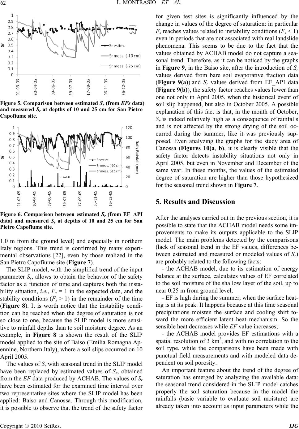

L. MONTRASIO ET AL.
62
Figure 5. Comparison between estimated Sr (from EFs data)
and measured Sr at depths of 10 and 25 cm for San Pietro
Capofiume site.
Figure 6. Comparison between estimated Sr (from EF_API
data) and measured Sr at depths of 10 and 25 cm for San
Pietro Capofiume site.
1.0 m from the ground level) and especially in northern
Italy regions. This trend is confirmed by many experi-
mental observations [22], even by those realized in the
San Pietro Capofiume site (Figure 7).
The SLIP model, with the simplified trend of the input
parameter Sr, allows to obtain the behavior of the safety
factor as a function of time and captures both the insta-
bility situation, i.e., Fs = 1 in the expected date, and the
stability conditions (Fs > 1) in the remainder of the time
(Figure 8). It is worth notice that the instability condi-
tion can be reached when the degree of saturation is not
so close to one, because the SLIP model is more sensi-
tive to rainfall depths than to soil moisture degree. As an
example, in Figure 8 is shown the result of the SLIP
model applied to the site of Baiso (Emilia Romagna Ap-
ennine, Northern Italy), where a soil slips occurred on 10
April 2005.
The values of Sr with seasonal trend in the SLIP model
have been replaced by estimated values of Sr, obtained
from the EF data produced by ACHAB. The values of Sr
have been estimated for the examined time interval over
two representative sites where the SLIP model has been
applied: Baiso and Canossa. Through this modification,
it is possible to observe that the trend of the safety factor
for given test sites is significantly influenced by the
change in values of the degree of saturation: in particular
Fs reaches values related to instability conditions (Fs < 1)
even in periods that are not associated with real landslide
phenomena. This seems to be due to the fact that the
values obtained by ACHAB model do not capture a sea-
sonal trend. Therefore, as it can be noticed by the graphs
in Figure 9, in the Baiso site, after the introduction of Sr
values derived from bare soil evaporative fraction data
(Figure 9(a)) and Sr values derived from EF_API data
(Figure 9(b)), the safety factor reaches values lower than
one not only in April 2005, when the historical event of
soil slip happened, but also in October 2005. A possible
explanation of this fact is that, in the month of October,
Sr is indeed relatively high as a consequence of rainfalls
and is not affected by the strong drying of the soil oc-
curred during the summer, like it was previously sup-
posed. Even analyzing the graphs for the study area of
Canossa (Figures 10(a, b), it is clearly visible that the
safety factor detects instability situations not only in
April 2005, but even in November and December of the
same year. In these months, the values of the estimated
degree of saturation are higher than those hypothesized
for the seasonal trend shown in Figure 7.
5. Results and Discussion
After the analyses carried out in the previous section, it is
possible to state that the ACHAB model needs some im-
provements to make its outputs applicable to the SLIP
model. The main problems detected by the comparisons
(lack of seasonal trend in the EF values, differences be-
tween estimated and measured or modeled values of Sr)
are probably related to the following facts:
- the ACHAB model, due to its estimation of energy
balance at the surface, calculates values of EF correlated
to the soil moisture of the shallow layer of the soil, up to
near 0.25 m from ground level;
- EF is high during the summer, when the surface heat-
ing is at its peak. It happens because at this time seasonal
precipitations moisten the surface and cooling shift to-
ward the more efficient latent heat mechanism. So the
sensible heat decreases while EF value increases;
- the ACHAB model provides EF estimations with a
spatial resolution of 3 km2, and with no correlation to the
soil type, while the comparisons have been made with
punctual field measurements and with modeled data de-
pendent on soil porosity.
An important feature about the trend of the degree of
saturation has emerged by analyzing the available data:
the seasonal trend considered in the SLIP model catches
properly the soil saturation because in the model the
rainfalls (basic variable to evaluate soil moisture) are
already taken into account as input parameters while the

L. MONTRASIO ET AL.
63
Figure 7. Comparison between experimental observations
of Sr at different soil depth in the San Pietro Capofiume site
and Sr considered changing with seasonal trend.
Figure 8.Behavior of the safety factor as a function of time
in the site of Baiso, with the simplified trend of Sr.
(a)
(b)
Figure 9. Trend of the safety factor as a function of time, in
the site of Baiso. Is highlighted the introduction of Sr values
obtained from EFs data (a) and from EF_API data (b).
(a)
(b)
Figure 10. Trend of the safety factor as a function of time in
the site of Canossa. Is highlighted the introduction of Sr
values obtained from EFs data (a) and from EF_API data
(b).
variable land surface temperature (that makes Sr vary
seasonally) is not considered as an input parameter of the
model and is introduced by means of the trend of the
degree of saturation.
In order to enable the use of ACHAB output for a
more accurate estimation of the degree of saturation,
which in its turn could be used in the SLIP model, the
results of the present work suggest the following im-
provements for future works:
- the relationship between evaporative fraction and
volumetric soil moisture content should be modified, on
the basis of field measurements, in order to take into ac-
count the real moisture content at higher depths;
- calibration parameters of ACHAB model have to be
modified dynamically (in time) in order to take into ac-
count seasonal weather conditions;
- ACHAB model could consider space-varying pa-
rameters to take into account different soil types.
6. Conclusions
Due to the need of rapid and reliable techniques for the
estimation of the degree of saturation of soils, which are
involved in rainfall-induced landslides, a new method of
soil moisture detection using a remote sensing technique
(the ACHAB system) has been analyzed, in order to

L. MONTRASIO ET AL.
64
evaluate the possibility of inserting the calculated values
in the model for characterizing the triggering mechanism
of shallow landslides (the SLIP model). To enable the
use of ACHAB processing for a more accurate estima-
tion of the degree of saturation, the ACHAB model
should be improved through appropriate spatio-temporal
parameters to provide estimation with a seasonal trend
for different kinds of soil. Developing these changes, the
ACHAB model results would be useful to determine the
Sr parameter and to take advantage of it in the SLIP
model, especially in its implementation on a platform for
a real-time territory control.
7. Acknowledgements
EF data were provided by the CIMA Foundation of
Savona and Protezione Civile Nazionale, while experi-
mental data of the degree of saturation were provided by
ARPA-SIM Emilia Romagna (Regional Agency for En-
vironmental Protection – Hydro-Meteorological Service).
The authors would like to express their gratitude to Dr. R.
Rudari, Dr. F. Tomei and Prof. M. Bittelli for their coop-
eration.
8. References
[1] L. Montrasio, “Stability Analysis of Soil Slip,” Proceed-
ings of International Conference Risk 2000, C. A. Breb-
bia, Ed., Wit Press, Southampton, 2000.
[2] L. Montrasio and R. Valentino, “Experimental Analysis
and Modelling of Shallow Landslides,” Landslides,
Springer, Vol. 4, No. 3, 2007, pp. 291-296.
[3] L. Montrasio and R. Valentino, “A Model for Triggering
Mechanisms of Shallow Landslide,” Natural Hazards
and Earth System Sciences, Vol. 8, No. 5, 2008, pp.
1149-1159.
[4] L. Montrasio, R. Valentino and G. L. Losi, “Rainfall-
Induced Shallow Landslides: A Model for the Triggering
Mechanism of Some Case Studies in Northern Italy,”
Landslides, Springer, Vol. 6, No. 3, 2009, pp. 241-251.
[5] L. Montrasio and R. Valentino, “X-SLIP: Un Modello per
l’innesco di Frane Indotte da Piogge, Fisicamente Basato,
Implementato su Piattaforma Experience,” Proceedings
of Annual Meeting of Italian Geotechnical Researchers,
IARG 2009 (in Italian), Roma, September 2009.
[6] R. Valentino, L. Montrasio, and G. L. Losi, “Modell-
azione Dell’innesco di Frane Superficiali Indotte da
Piogge: Dalla Scala Locale a Quella Regionale,” Pro-
ceedings of Annual Meeting of Italian Geotechnical
Researchers, IARG 2009 (in Italian), Roma, September
2009.
[7] M. Caruso, “Una Metodologia Teorica, Sperimentale e
Numerica per la Previsione del Bilancio Idrico nei
Terreni Superficiali non Saturi,” Ph.D. Dissertation, Uni-
versity of Parma, Parma, 2007.
[8] B. R. Scanlon, R. W. Healy and P. G. Cook, “Choosing
Appropriate Techniques for Quantifying Groundwater Re-
charge,” Hydrogeology Journal, Vol. 10, 2002, pp. 18-39.
[9] G. Boni, F. Castelli and D. Entekabi, “Sampling Strate-
gies and Assimilation of Ground Temperature for the Es-
timation of Surface Energy Balance Components,” IEEE
Transactions on Geoscience and Remote Sensing, Vol. 39,
No. 1, 2001, pp. 165-172.
[10] F. Caparrini, F. Castelli and D. Entekabi “Variational
Estimation of Soil and Vegetation Turbulent Transfer and
Heat Flux Parameters from Sequences of Multisensory
Imagery,” Water Resources Research, Vol. 40, No.
W12515, 2004, pp. 15-25.
[11] F. Caparrini, F. Castelli, D. Entekabi and L. Campo,
“Sequential Assimilation of Land Temperature for Moni-
toring Surface Components of the Hydrologic Cycle,”
EUMETSAT Meteorological Satellite Conference, Hel-
sinki, June 2006.
[12] C. H. B. Priestley and R. J. Taylor, “On the Assessment
of Surface Heat Flux and Evaporation Using Large-Scale
Parameters,” Monthly Weather Review, Vol. 100, No. 2,
1972, pp. 81-92.
[13] J. L. Monteith, Principles of Environmental Physics,
Edward Arnold Press, London, 1973.
[14] W. J. Shuttleworth, R. J. Gurney, A. Y. Hsu and J. P.
Ormsby, “FIFE: The Variation in Energy Partition at
Surface Flux Sites,” In: A. Rango, Ed., Remote Sensing
and Large-Scale Processes, Proceedings of the IAHS
Third International Assembly, IAHS Publication, Balti-
more, Vol. 186, 1989, pp. 67-74.
[15] F. Sini, “Satellite Data Assimilation for the Estimation of
Surface Energy Fluxes,” Ph.D. Dissertation, University of
Basilicata, Potenza, 2005.
[16] A. Pistocchi, F. Bouraoui and M. Bittelli, “A Simplified
Parameterization of the Monthly Topsoil Water Budget,”
Water Resources Research, Vol. 44, No. W12440, 2008.
[17] E. A. Smith, A. Y. Hsu, W. L. Crosson, R. T. Field, L. J.
Fritschen, R. J. Gurney, E. T. Kanemasu, W. P. Kustas, D.
Nie, W. J. Shuttleworth, J. B. Stewart, S. B. Verma, H. L.
Weaver and M. L. Wesely, “Area-Averaged Surface
Fluxes and their Time-Space Variability over the FIFE
Experimental Domain,” Journal of Geophysical Research,
Vol. 97, No. D17, 1992, pp. 18599-18622.
[18] W. G. M. Bastiaanssen, H. Pelgrum, P. Droogers, H. A. R.
de Bruin and M. Menenti, “Area-Average Estimates of
Evaporation, Wetness Indicators and Topsoil Moisture
during Two Golden Days in EFEDA,” Agricultural and
Forest Meteorology, Vol. 87, No. 2, 1997, pp. 119-137.
[19] W. G. M. Bastiaanssen, D. J. Molden and I. W. Makin,
“Remote Sensing for Irrigated Agriculture: Examples
from Research of Possible Applications,” Agricultural
Water Management, Vol. 46, No. 2, 2000, pp. 137-155.
[20] M. Ahmad and W. Bastiaanssen, “Retrieving Soil Mois-
ture Storage in the Unsaturated Zone Using Satellite Im-
agery and Bi-Annual Phreatic Surface Fluctuations,” Ir-
rigation and Drainage Systems, Vol. 17, No. 3, 2003, pp.
141-161.

L. MONTRASIO ET AL.
65
[21] C. Scott, W. Bastiaanssen and M. Ahmad, “Mapping
Root Zone Soil Moisture Using Remotely Sensed Optical
Imagery,” Journal of Irrigation and Drainage Engi-
neering, ASCE, Vol. 129, No. 5, 2003, pp. 326-335.
[22] C. Quintavalla, “Valutazione del Grado di Saturazione in
Terreni Superficiali per l’analisi di Stabilità di Pendii in
Terra,” MSc Thesis (in Italian), University of Parma,
Faculty of Engineering, Parma, 2006.