1. Introduction
Malliavin calculus is the infinite-dimensional differential calculus on the Wiener space in order to give a probabilistic proof of Hölmander’s theorem. It has been developed as a tool in mathematical finance. In 1999, Founié et al. [1] gave a new method for more efficient computation of Greeks which represent sensitivities of the derivative price to changes in parameters of a model under consideration, by using the integration by parts formula related to Malliavin calculus. Following their works, more general and efficient applications to computation of Greeks have been introduced by many authors (see [2] [3] [4]). They often considered this method for tractable models typified by the Black-Scholes model.
In the Black-Scholes model, an underlying asset  is assumed to follow the stochastic differential equation
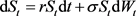 , where r and
  respectively imply the risk free interest rate and the volatility. The Black-Scholes model seems standard in business. The reason is that this model has the analytic solution for famous options, so it is fast to calculate prices of derivatives and risk parameters (Greeks) and easy to evaluate a lot of deals and the whole portfolios and to manage the risk. However, the Black-Scholes model has a defect that this model assumes that volatility is a constant.
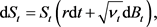
In the actual financial market, it is observed that volatility fluctuates. However, the Black-Scholes model does not suppose the prospective fluctuation of volatility, so when we use the model there is a problem that we would underestimate prices of options. Hence, more accurate models have been developed. One of the models is the stochastic volatility model. One of merits to consider this model is that even if prices of derivatives such as the European options are not given for any strike and maturity, we can grasp the volatility term structure. In particular, the Heston model, which is introduced in [5], is one of the most popular stochastic volatility models. This model assumes that the underlying asset  and the volatility
  follow the stochastic differential equations
 (1.1)
(1.1)
 (1.2)
(1.2)
where  and
and  denote correlated Brownian motion s. In the Equation (1.2),
  ,
,  and
and  imply respectively the rate of mean reversion (percentage drift), the long-run mean (equilibrium level) and the volatility of volatility. This volatility model is called the Cox-Ingersoll-Ross model and more complicated than the Black-Scholes model. We have not got the analytic solution yet.
However, even this model cannot grasp fluctuation of volatility accurately. In 2006 (see [6]), Andersen and Piterbarg generalized the Heston model. They extended the volatility process of (1.2) to
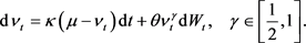 (1.3)
(1.3)
This model is called the constant elasticity of variance model (we will often shorten this model as the CEV model). Naturally, in the case , the volatility model (1.3) is more complicated than the volatility model (1.2).
Here, consider the European call option and let  is a payoff function. Then we can estimate the option price by the following formula
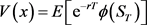 . However, the computation of Greeks is much important in the risk-management.
A Greek is given by  where
where  is one of parameters needed to compute
the price, such as the initial price, the risk free interest rate, the volatility and the maturity etc.. Most of financial institutions have calculated Greeks by using finite-difference methods but there are some demerits such that the results depend on the approximation parameters. More than anything, the methods need the assumption that the payoff function ![]() is differentiable. However, in business they often consider the payoff functions such as
is differentiable. However, in business they often consider the payoff functions such as ![]() or
or![]() . Here we need Malliavin calculus. In 1999 Founié et al. in [1] gave the new methods for Greeks. To come to the point, they calculated Greeks by the following
. Here we need Malliavin calculus. In 1999 Founié et al. in [1] gave the new methods for Greeks. To come to the point, they calculated Greeks by the following
formula![]() . We can calculate this even if
. We can calculate this even if ![]() is
is
polynomial growth. Instead, we need the Malliavin differentiability of![]() .
.
The solution ![]() satisfying the stochastic differential equation with Lipschitz continuous coefficients is known as Malliavin differentiable. Hence we can easily verify that the Black-Scholes model is Malliavin differentiable. However the
satisfying the stochastic differential equation with Lipschitz continuous coefficients is known as Malliavin differentiable. Hence we can easily verify that the Black-Scholes model is Malliavin differentiable. However the
diffusion coefficient ![]() is neither differentiable at
is neither differentiable at ![]() nor Lipschitz
nor Lipschitz
continuous and then we cannot find whether the CEV-type Heston model is Malliavin differentiable or not. In [7], Alos and Ewald proved that the volatility
process (1.2), that is the case where ![]() of (1.3), was Malliavin differentiable and gave the explicit expression for the derivative. However, in the case
of (1.3), was Malliavin differentiable and gave the explicit expression for the derivative. However, in the case![]() , we cannot simply prove the Malliavin differentiability in the exact same way.
, we cannot simply prove the Malliavin differentiability in the exact same way.
In this paper we concentrate on the case![]() , that is, we extend the
, that is, we extend the
results in [7] and give the explicit expression for the derivative. Moreover we consider the CEV-type Heston model and give the formula to compute Greeks.
2. Summary of Malliavin Calculus
We give the short introduction of Malliavin calculus on the Wiener space. For further details, refer to [8].
2.1. Malliavin Derivative
We consider a Brownian motion ![]() (in the sequel, we often denote
(in the sequel, we often denote ![]() by
by![]() ) on a complete filtered probability space
) on a complete filtered probability space ![]() where
where ![]() is the filtration generated by
is the filtration generated by![]() , and the Hilbert space
, and the Hilbert space![]() . When fixing
. When fixing![]() , we can consider
, we can consider![]() . Then the Itô integral of
. Then the Itô integral of
![]() is constructed as
is constructed as ![]() on
on![]() . We denote
. We denote
by ![]() the set of infinitely continuously differentiable functions
the set of infinitely continuously differentiable functions ![]() such that f and all its partial derivatives have polynomial growth. Let S be the space of smooth random variables expressed as
such that f and all its partial derivatives have polynomial growth. Let S be the space of smooth random variables expressed as
![]() (2.1)
(2.1)
where ![]() and
and ![]() where
where![]() ,
,![]() . We denote by
. We denote by ![]() the set of infinitely continuously differentiable functions
the set of infinitely continuously differentiable functions ![]() such that f has compact support. Moreover we denote by
such that f has compact support. Moreover we denote by ![]() the set of infinitely continuously differentiable functions
the set of infinitely continuously differentiable functions ![]() such that ƒ and all of its partial derivatives are bounded. Denote by
such that ƒ and all of its partial derivatives are bounded. Denote by ![]() and
and ![]() respectively, the spaces of smooth random variables of the form (2.1) such that
respectively, the spaces of smooth random variables of the form (2.1) such that ![]() and
and![]() . We can find that
. We can find that ![]() and
and ![]() is a linear subspace of and dense in
is a linear subspace of and dense in ![]() for all
for all![]() . We use the notation
. We use the notation ![]() in the
in the
sequal. We define the derivative operator D, so called the Malliavin derivative operator.
Definition 2.1. (Malliavin derivative) The Malliavin derivative ![]() of a smooth random variable expressed as (2.1) is defined as the H-valued random variable given by
of a smooth random variable expressed as (2.1) is defined as the H-valued random variable given by
![]() (2.2)
(2.2)
We sometimes omit to write the subscript t.
Since ![]() is dense in
is dense in![]() , we will define the Malliavin derivative of a general
, we will define the Malliavin derivative of a general ![]() by means of taking limits. We will now prove that the Malliavin derivative operator
by means of taking limits. We will now prove that the Malliavin derivative operator ![]() is closable. Please refer to [8] for proves of the following results.
is closable. Please refer to [8] for proves of the following results.
Lemma 2.1. We have![]() , for
, for ![]() and
and![]() .
.
Lemma 2.2. For any![]() , the Malliavin derivative operator
, the Malliavin derivative operator ![]() is closable.
is closable.
For any![]() , we denote by
, we denote by ![]() the domain of D in
the domain of D in ![]() and then it is the closure of
and then it is the closure of ![]() by the norm
by the norm
![]() (2.3)
(2.3)
Note that ![]() is a Hilbert space with the scalar product
is a Hilbert space with the scalar product ![]() . Moreover, the Malliavin derivative
. Moreover, the Malliavin derivative ![]() is regarded as a stochastic process defined almost surely with the measure
is regarded as a stochastic process defined almost surely with the measure ![]() where u is a Lebesgue measure in
where u is a Lebesgue measure in![]() . Indeed, we can observe
. Indeed, we can observe
![]() (2.4)
(2.4)
The following result will become a very important tool.
Lemma 2.3. Suppose that a sequence ![]() converges to F in
converges to F in![]() . Then F belongs to
. Then F belongs to ![]() and the sequence
and the sequence ![]() converges to DF in the weak topology of
converges to DF in the weak topology of![]() .
.
Similarly, we define the k-th Malliavin derivative of F, ![]() , as a
, as a ![]() -measurable stochastic process defined
-measurable stochastic process defined ![]() -almost surely and the operator
-almost surely and the operator ![]() is closable from
is closable from ![]() for any
for any ![]() and
and![]() . As with the Malliavin derivative D, from the closability of
. As with the Malliavin derivative D, from the closability of![]() , we can define the domain
, we can define the domain ![]() of the operator
of the operator ![]() in
in ![]() as the completion of
as the completion of ![]() with the norm
with the norm
![]() (2.5)
(2.5)
Moreover we define ![]() as
as![]() . We will now prove the chain rule and refer to the ( [8], Proposition 1.2.4) for details.
. We will now prove the chain rule and refer to the ( [8], Proposition 1.2.4) for details.
Lemma 2.4. For![]() , let
, let ![]() and
and ![]() be a Lipschitz function with bounded partial derivatives, and then we have
be a Lipschitz function with bounded partial derivatives, and then we have ![]() and
and
![]() (2.6)
(2.6)
2.2. Skorohod Integral
For ![]() satisfing
satisfing![]() , the adjoint
, the adjoint ![]() of the operator D which is closable and has the domain on
of the operator D which is closable and has the domain on ![]() should be closable but with the domain contained in
should be closable but with the domain contained in![]() . Focus on the case
. Focus on the case![]() . We can define the divergence operator
. We can define the divergence operator ![]() so called the Scorohod integral which is the adjoint of the operator D such as
so called the Scorohod integral which is the adjoint of the operator D such as
![]() (2.7)
(2.7)
Definition 2.2 (Skorohod integral). Let![]() . If for all
. If for all![]() , we can have
, we can have
![]() (2.8)
(2.8)
where c is some constant depending on u, then u is called to belong to the domain![]() . Moreover if
. Moreover if![]() , then we have that
, then we have that ![]() belongs to
belongs to ![]() and the duality relation
and the duality relation![]() , for all
, for all![]() .
.
We can get the following results.
Lemma 2.5. Let ![]() and
and ![]() satisfy
satisfy![]() . And then we have that
. And then we have that ![]() belongs to
belongs to ![]() and
and![]() .
.
Lemma 2.6. Let ![]() be an
be an ![]() -adapted stochastic process then
-adapted stochastic process then ![]() and
and![]() .
.
We give one of famous properties of![]() . The following property implies the relationship between the Malliavin derivative and the Skorohod integral. Denote by
. The following property implies the relationship between the Malliavin derivative and the Skorohod integral. Denote by ![]() the class of processes
the class of processes ![]() such that
such that
![]() for almost all t and there exists a measurable version of the two
for almost all t and there exists a measurable version of the two
variable processes ![]() satisfying
satisfying![]() .
.
Lemma 2.7. Let ![]() satisfy that
satisfy that ![]() and that
and that ![]() . We have then that
. We have then that ![]() belongs to
belongs to ![]() and
and
![]() (2.9)
(2.9)
The following result is applied to calculate Greeks. For further details, refer to ( [8], Chapter 6).
Lemma 2.8. Let![]() . Suppose that an random variable
. Suppose that an random variable ![]() satisfy
satisfy ![]() a.s. and
a.s. and![]() . For any continuously differentiable function f with bounded derivatives, we have
. For any continuously differentiable function f with bounded derivatives, we have
![]()
where![]() .
.
2.3. Malliavin Calculus for Stochastic Differential Equations
Consider ![]() and
and![]() . Let
. Let ![]() be the m-dimensional
be the m-dimensional
Brownian motion on filtered probability space ![]() where P is the n-dimensional Wiener measure and F is the completion of the σ-field of
where P is the n-dimensional Wiener measure and F is the completion of the σ-field of ![]() with P. And then
with P. And then ![]() is the underlying Hilbert space. We consider the solution
is the underlying Hilbert space. We consider the solution ![]() of the following n-dimensional stochastic differential equation for all
of the following n-dimensional stochastic differential equation for all ![]()
![]() (2.10)
(2.10)
where ![]() and
and ![]() satisfy the following : there is a positive constant
satisfy the following : there is a positive constant ![]() such that
such that
![]() (2.11)
(2.11)
![]() (2.12)
(2.12)
Here ![]() is the columns of the matrix
is the columns of the matrix![]() . We can have the following result related to the uniqueness and refer to ( [8], Lemma 2.2.1) for the detail.
. We can have the following result related to the uniqueness and refer to ( [8], Lemma 2.2.1) for the detail.
Theorem 2.1. There is a unique n-dimensional, continuous and ![]() -adapted stochastic process
-adapted stochastic process ![]() satisfying the stochastic differential Equation (2.10) with
satisfying the stochastic differential Equation (2.10) with![]() , for all
, for all![]() .
.
In the case the coefficients are Lipschitz, the solution ![]() belongs to
belongs to![]() .
.
Theorem 2.2. Assume that coefficients are Lipschitz continuous of the stochastic differential Equation (2.10). Then the solution ![]() belongs to
belongs to ![]() for all
for all ![]() and
and ![]() and satisfies
and satisfies
![]() (2.13)
(2.13)
Moreover the derivative ![]() satisfies the following
satisfies the following
![]() (2.14)
(2.14)
for ![]() a.e., and
a.e., and ![]() for
for ![]() a.e.. Here
a.e.. Here ![]() denotes the Malliavin derivative for
denotes the Malliavin derivative for![]() .
.
Let ![]() be the solution of the following stochastic differential equation
be the solution of the following stochastic differential equation
![]() (2.15)
(2.15)
where ![]() denotes a 1-dimensional Brownian motion. Assume that
denotes a 1-dimensional Brownian motion. Assume that![]() . We let
. We let ![]() be the first variation of
be the first variation of![]() , that is,
, that is,![]() . We can easily have that
. We can easily have that ![]() satisfies the folloing
satisfies the folloing
![]() (2.16)
(2.16)
Considering this as a stochastic differential equation for![]() , we can have the following solution
, we can have the following solution
![]() (2.17)
(2.17)
The following results will also be useful to calculate Greeks later.
Lemma 2.9. Under the above conditions, we can have ![]() .
.
Let ![]() be a continuous function in H such that
be a continuous function in H such that![]() .
.
Lemma 2.10. Under the above conditions, we can have ![]() .
.
Theorem 2.3. For any ![]() of polynomial growth, we have
of polynomial growth, we have ![]() where
where![]() .
.
For the more general case, the same result is proved as below. Let ![]() denote the solution of the following n-dimensional stochastic differential equation just like as (2.10)
denote the solution of the following n-dimensional stochastic differential equation just like as (2.10)
![]() (2.18)
(2.18)
where ![]() denotes m-dimensional Brownian motion. For the sake of simplification, we assume that
denotes m-dimensional Brownian motion. For the sake of simplification, we assume that![]() .
.
Theorem 2.4. Suppose that the diffusion coefficient ![]() is invertible and that
is invertible and that![]() , for some
, for some![]() , where Y denotes the first variation
, where Y denotes the first variation
process, that is,![]() . Let
. Let ![]() be a random variable which does not depend on the initial condition x. Then for all measurable function
be a random variable which does not depend on the initial condition x. Then for all measurable function ![]() with polynomial growth we have
with polynomial growth we have![]() , where
, where ![]() is an
is an ![]() -adapted process satisfying
-adapted process satisfying![]() ,
,
![]() (2.19)
(2.19)
and ![]() denotes the adjoint to the Malliavin derivative with respect to a Brownian motion
denotes the adjoint to the Malliavin derivative with respect to a Brownian motion![]() .
.
The following theorem introduced in [9] is useful. From now on, we will now denote by ![]() the once derivative with respect to t, by
the once derivative with respect to t, by ![]() the once derivative with respect to x and by
the once derivative with respect to x and by ![]() the second derivative with respect to x.
the second derivative with respect to x.
Theorem 2.5. Consider a stochastic process ![]() satisfying the 1-dimensional stochastic differential equation
satisfying the 1-dimensional stochastic differential equation
![]() (2.20)
(2.20)
where ![]() denotes a Brownian motion and the coefficients
denotes a Brownian motion and the coefficients ![]() and
and ![]() satisfy the linear growth condition and the Lipschitz condition. Moreover, we assume that
satisfy the linear growth condition and the Lipschitz condition. Moreover, we assume that ![]() is positive and bounded away from 0, and that
is positive and bounded away from 0, and that ![]() and
and ![]() are bounded for all
are bounded for all![]() . Then
. Then ![]() belongs to
belongs to ![]() and the derivative is given by
and the derivative is given by
![]() (2.21)
(2.21)
for ![]() and
and ![]() for
for![]() .
.
Proof. We omit the proof. For further details, refer to (Theorem 2.1 [9]).
3. Mean-Reverting CEV Model
Following the construction in [7], we will now prove that the mean-reverting constant elasticity of variance model is Malliavin differentiable. The mean-reverting CEV model follows the stochastic differential equation
![]() (3.1)
(3.1)
with ![]() and where
and where![]() ,
, ![]() and
and![]() . In [7], Alos and Ewald proved the Malliavin differentiability of the case
. In [7], Alos and Ewald proved the Malliavin differentiability of the case ![]() of (3.1). In the case, the function
of (3.1). In the case, the function
![]() is neither continuously differentiable in 0 nor Lipschitz continuous so they circumvented various problems by some transforming and approximating.
is neither continuously differentiable in 0 nor Lipschitz continuous so they circumvented various problems by some transforming and approximating.
However, in the case![]() , there are more complex problems. Following [7], we will extend their results.
, there are more complex problems. Following [7], we will extend their results.
3.1. Existence and Uniqueness
We will now prove that the solution to (3.1) not only exists uniquely but is also positive a.s.
Lemma 3.1. There exists a unique strong solution to (3.1) which satisfies![]() . Moreover, let
. Moreover, let ![]() with
with![]() . Then we have
. Then we have![]() .
.
Proof. Instead of (3.1), consider the following
![]() (3.2)
(3.2)
If we have concluded that the unique strong solution of (3.2) is positive a.s., then (3.2) coincides with (3.1). The existence of non-explosive weak solution for (3.2) follows from the continuity and the sub-linear growth condition of drift and diffusion coefficients. Moreover, from ( [10], Proposition 5.3.20, Corollary 5.3.23), we have the pathwise uniqueness. From ( [10], Proposition 5.2.13), we can verify that the pathwise uniqueness holds for (3.2).
We will now prove that the second claim is true. Let
![]() with
with![]() . In order to use ( [10], Theorem 5.5.29), we verify that for a fixed number
. In order to use ( [10], Theorem 5.5.29), we verify that for a fixed number![]() ,
, ![]() where
where
![]() is defined as
is defined as![]() . Since we have known
. Since we have known
that the solution ![]() of (3.2) does not explode at
of (3.2) does not explode at![]() , if we could prove that the above formula holds, we can claim that
, if we could prove that the above formula holds, we can claim that![]() , that is,
, that is,![]() . We can assume without restriction that
. We can assume without restriction that ![]() and let
and let![]() . Then we have
. Then we have
![]() (3.3)
(3.3)
Letting![]() , we can calculate
, we can calculate![]() . From the last inequality, there exists a constant
. From the last inequality, there exists a constant ![]() satisfying the following inequality and then we have as
satisfying the following inequality and then we have as![]() ,
,
![]() (3.4)
(3.4)
3.2. Lp-Integrability
Consider the Stochastic Differential Equation
![]() (3.5)
(3.5)
with![]() , where b is such that
, where b is such that ![]() and satisfies the Lipschitz condition,
and satisfies the Lipschitz condition, ![]() and
and![]() . The following lemma ensures the existence of its moments of any order.
. The following lemma ensures the existence of its moments of any order.
Lemma 3.2. Consider the solution of the (3.5). For any![]() , we have
, we have ![]() and
and![]() .
.
Proof. At first we consider the positive moments. We define the stopping time ![]() with
with![]() . By Itô’s formula,
. By Itô’s formula,
![]() (3.6)
(3.6)
From the Lipschitz condition of the drift function![]() , there exists a positive constant K which satisfies
, there exists a positive constant K which satisfies![]() . By the above inequality and Young’s inequality, we have
. By the above inequality and Young’s inequality, we have
![]() (3.7)
(3.7)
By Gronwall’s lemma, we can have![]() , where both C and
, where both C and ![]() do not depend on n. As
do not depend on n. As![]() , we can obtain the result. Next we consider
, we can obtain the result. Next we consider
the negative moments. Define the stopping time as![]() , with
, with![]() . By Itô’s formula, we have
. By Itô’s formula, we have
![]() (3.8)
(3.8)
Taking the expectation and using the Fubini’s theorem, we have
![]() (3.9)
(3.9)
Here let![]() , then we can easily evaluate the boundedness for any
, then we can easily evaluate the boundedness for any ![]()
![]() (3.10)
(3.10)
Summarizing the calculation, we have![]() , and from Gronwall’s lemma we finally have
, and from Gronwall’s lemma we finally have![]() . Taking the limit
. Taking the limit![]() , then
, then ![]() so we have
so we have ![]() . Hence we can deduce the result.
. Hence we can deduce the result.
Remark 1. Since the CEV model satisfies the assumptions of Lemma 3.2, so the result holds for the CEV model.
3.3. Transformation and Approximation
We consider the process transformed as![]() . By Itô’s formula, we have
. By Itô’s formula, we have
![]() (3.11)
(3.11)
with![]() . If
. If ![]() is the solution of the stochastic differential Equation (3.11), then we can prove that
is the solution of the stochastic differential Equation (3.11), then we can prove that ![]() is also the solution of the stochastic differential Equation (3.1) satisfying the initial condition
is also the solution of the stochastic differential Equation (3.1) satisfying the initial condition![]() . By this transformation, we can replace (3.1) by (3.11) with the constant volatility term. In order to use Theorem 2.5, we must approximate
. By this transformation, we can replace (3.1) by (3.11) with the constant volatility term. In order to use Theorem 2.5, we must approximate ![]() and
and ![]() by the Lipschitz
by the Lipschitz
continuous functions, respectively. For all![]() , define the continuously differentiable functions
, define the continuously differentiable functions ![]() and
and ![]() as
as
![]() (3.12)
(3.12)
![]() (3.13)
(3.13)
For the functions ![]() and
and![]() , we can easily verify that for all
, we can easily verify that for all![]() ,
, ![]() and
and ![]() and then we have that for all
and then we have that for all![]() ,
, ![]() and
and![]() . Moreover, note that for all
. Moreover, note that for all![]() ,
, ![]() and
and![]() . Define our approximations
. Define our approximations ![]() as the stochastic process following the stochastic differential equation
as the stochastic process following the stochastic differential equation
![]() (3.14)
(3.14)
with ![]() for all
for all![]() . The coefficients of the Equation (3.14) are Lipschitz continuous because we can have for all
. The coefficients of the Equation (3.14) are Lipschitz continuous because we can have for all![]() ,
,
![]() (3.15)
(3.15)
We will prove that ![]() converges to
converges to ![]() in
in![]() . First we prove that
. First we prove that ![]() converges to
converges to ![]() pointwise.
pointwise.
Lemma 3.3. The sequence ![]() converges to
converges to ![]() a.s., for all
a.s., for all![]() .
.
Proof. Define for all ![]() the stopping time as
the stopping time as ![]() with
with![]() . By the definition of
. By the definition of![]() ,
, ![]() , and
, and![]() , we have
, we have
![]() (3.16)
(3.16)
By Gronwall’s lemma, ![]() for
for ![]() and by Lemma 3.1 and the fact that
and by Lemma 3.1 and the fact that ![]() for
for![]() , we have
, we have ![]() a.s. so
a.s. so ![]() for all
for all![]() .
.
Next we prove that there exist square integrable processes ![]() and
and ![]() with
with ![]() for all
for all![]() . Actually, we will see that
. Actually, we will see that ![]() is
is![]() . Before starting with the proof, we prove the following inequality.
. Before starting with the proof, we prove the following inequality.
Lemma 3.4. For ![]() and
and![]() , let
, let![]() . We have, for
. We have, for![]() ,
,
![]() (3.17)
(3.17)
Proof. By differentiating![]() , we can easily have the result.
, we can easily have the result.
Consider ![]() and
and ![]() in the above inequality, then we can have the below result.
in the above inequality, then we can have the below result.
Lemma 3.5. Let ![]() be the solution of the following stochastic differential equation
be the solution of the following stochastic differential equation
![]() (3.18)
(3.18)
with![]() , where
, where![]() . Then
. Then ![]() a.s. for all
a.s. for all![]() .
.
Proof. From the definitions of ![]() and
and![]() ,
, ![]() for all
for all
![]() , that is, the drift coefficient of
, that is, the drift coefficient of ![]() is smaller than one of
is smaller than one of![]() . By Yamada-Watanabe’s comparison lemma (see [10], Proposition 5.2.18) and Lemma 3.1, we have
. By Yamada-Watanabe’s comparison lemma (see [10], Proposition 5.2.18) and Lemma 3.1, we have ![]() a.s.
a.s.
We prove the second inequality. In order to use Yamada-Watanabe’s comparison lemma, we must prove that, for![]() ,
, ![]() . Let
. Let ![]() . We can easily verify
. We can easily verify ![]() , for
, for ![]() and
and ![]() for
for![]() . For all
. For all![]() , we have
, we have
![]() (3.19)
(3.19)
![]() (3.20)
(3.20)
Then there is a constant ![]() with
with ![]() for all
for all ![]() and
and ![]() for all
for all![]() . For
. For![]() ,
, ![]() is decreasing for all
is decreasing for all![]() . Then
. Then ![]() and
and ![]() imply for all
imply for all![]() ,
, ![]() , that is, for
, that is, for ![]()
![]() (3.21)
(3.21)
By Yamada-Watanabe’s comparison lemma, we have ![]() a.s.
a.s.
Theorem 3.1. For all![]() , the sequence
, the sequence ![]() converges to
converges to ![]() in
in![]() .
.
Proof. From Lemma 3.5, we have![]() . Lemma 3.2 implies
. Lemma 3.2 implies![]() . Moreover, the Ornstein-Uhlenbeck process
. Moreover, the Ornstein-Uhlenbeck process![]() . By the dominated convergence theorem we can have the convergence.
. By the dominated convergence theorem we can have the convergence.
3.4. Malliavin Differentiability
We will prove the Malliavin differentiability of both ![]() and
and![]() . To do this, we consider our approximation sequence
. To do this, we consider our approximation sequence![]() . The approximating stochastic differential Equation (3.14) of
. The approximating stochastic differential Equation (3.14) of ![]() satisfies the assumption of Theorem 2.5, so we can prove the Malliavin differentiability of
satisfies the assumption of Theorem 2.5, so we can prove the Malliavin differentiability of![]() .
.
Lemma 3.6. ![]() belongs to
belongs to ![]() and we have
and we have
![]() (3.22)
(3.22)
for![]() , and
, and ![]() for
for![]() .
.
Proof. By Theorem 2.5, we have the result.
We will now prove the Malliavin differentiability of![]() . To start with, we prove some useful lemmas.
. To start with, we prove some useful lemmas.
Lemma 3.7. For ![]() and
and![]() , let
, let![]() , then for
, then for ![]() we have
we have
![]() (3.23)
(3.23)
Proof. By differentiating ![]() we can easily have the result.
we can easily have the result.
By Lemma 3.7, considering the case where ![]() and
and![]() , we have for
, we have for![]() ,
,
![]() (3.24)
(3.24)
We have for![]() ,
,
![]() (3.25)
(3.25)
so there exists a constant ![]() such that for all
such that for all![]() ,
, ![]() . Hence, for
. Hence, for![]() , we have
, we have![]() , for all
, for all![]() . Note that
. Note that ![]() is independent of
is independent of![]() . By this inequality, we have the following result.
. By this inequality, we have the following result.
Lemma 3.8. We have for all ![]() and
and![]() ,
,
![]() (3.26)
(3.26)
Proof. When![]() ,
, ![]() so the result follows. Moreover when
so the result follows. Moreover when![]() , putting above results together, we obtain the result.
, putting above results together, we obtain the result.
Putting the scenarios together, we can prove the following.
Theorem 3.2. ![]() belongs to
belongs to ![]() and we have
and we have
![]() (3.27)
(3.27)
for![]() , and
, and ![]() for
for![]() .
.
Proof. We have proved that ![]() in
in ![]() and
and![]() . Moreover, by Lemma 3.8, we have
. Moreover, by Lemma 3.8, we have![]() . Here
. Here ![]() converges to
converges to ![]() also pointwise, we can conclude that
also pointwise, we can conclude that ![]() converges to
converges to
![]() . Using the bounded
. Using the bounded
convergence theorem, we can have that ![]() converges to G in
converges to G in![]() . Hence by Lemma 2.4, we can conclude that
. Hence by Lemma 2.4, we can conclude that ![]() and
and![]() .
.
Moreover we can prove the following Malliavin differentiability in more detail.
Theorem 3.3. For all![]() ,
, ![]() belongs to
belongs to![]() , that is,
, that is, ![]() belongs to
belongs to![]() .
.
Proof. We only have to prove that![]() . We have
. We have
![]() (3.28)
(3.28)
Hence we can conclude that![]() .
.
By the chain rule, we can conclude that ![]() is also Malliavin differentiable.
is also Malliavin differentiable.
Theorem 3.4. For all![]() ,
, ![]() belongs to
belongs to ![]() and the Malliavin derivative is given by
and the Malliavin derivative is given by
![]() (3.29)
(3.29)
for![]() , and
, and ![]() for
for![]() .
.
Proof. Consider only the case where![]() . Similarly, we can easily prove the case where
. Similarly, we can easily prove the case where![]() . We have shown that
. We have shown that ![]() and
and![]() . By Lemma 2.5, we have
. By Lemma 2.5, we have
![]() (3.30)
(3.30)
For all![]() , using Young’s inequality and the fact
, using Young’s inequality and the fact ![]() and
and![]() , we can prove that
, we can prove that ![]() belongs to
belongs to![]() . Indeed, we have
. Indeed, we have
![]() (3.31)
(3.31)
4. CEV-Type Heston Model and Greeks
We will now consider the CEV-type Heston model and Greeks. Fournié et al. introduced new numerical methods for calculating Greeks using Malliavin calculus for the first time in 1999 (see [1]). We call this methods Malliavin Monte-Carlo methods. They focused on models with Lipschitz continuous coefficients, and then a lot of researchers have considered Malliavin Monte-Carlo methods to compute Greeks. However, lately, there is need to focus on models with non-Lipschitz coefficients such as stochastic volatility models. In 2008, Alos and Ewald proved that the Cox-Ingersoll-Ross model was Malliavin differentiable (see [7]). We apply Malliavin calculus for calculating Greeks of the CEV-type Heston model which is one of the important in business but mathematically complex models. Basically, we consider the European option but we can easily extend this result to other options.
4.1. Greeks
We introduce the concept of Greeks. For example, consider a European option with payoff function ![]() depending on the final value of the underlying asset
depending on the final value of the underlying asset ![]() where
where ![]() denotes a stochastic process expressing the asset and T denotes the maturity of the option. The price V is given by
denotes a stochastic process expressing the asset and T denotes the maturity of the option. The price V is given by ![]() where r is the risk-free rate. We can estimate this by Monte-Carlo simulations. Greeks are derivatives of the option price V with respect to the parameters of the model. Greeks are the useful measure for the portfolio risk management by traders in financial institutions. Most of financial institutions estimate Greeks by finite difference methods. However, there are some demerits. For examples, the numerical results depend on the approximation parameters and, in the case where
where r is the risk-free rate. We can estimate this by Monte-Carlo simulations. Greeks are derivatives of the option price V with respect to the parameters of the model. Greeks are the useful measure for the portfolio risk management by traders in financial institutions. Most of financial institutions estimate Greeks by finite difference methods. However, there are some demerits. For examples, the numerical results depend on the approximation parameters and, in the case where ![]() is not differentiable, this methods do not work well. In [1], Founié et al. gave the new methods to circumvent these problems. The idea is that we calculate Greeks by multiplying the weight, so-called Malliavin weight, as following
is not differentiable, this methods do not work well. In [1], Founié et al. gave the new methods to circumvent these problems. The idea is that we calculate Greeks by multiplying the weight, so-called Malliavin weight, as following
![]() (4.1)
(4.1)
This methods are much useful since we do not require the differentiability of the payoff function![]() . Instead, there is need to assume that the underlying assert
. Instead, there is need to assume that the underlying assert ![]() is Malliavin differentiable. From Theorem 2.2, we find that the solution of the stochastic differential equation with Lipschitz continuous coefficients are Malliavin differentiable. However, if a model under consideration becomes more complex just like the CEV-type Heston model, we could not apply this Malliavin methods. Through Section 4, we consider the Malliavin differentiability of the CEV-type Heston model in order to give formulas for Greeks, in particular, Delta and Rho. Here, Delta
is Malliavin differentiable. From Theorem 2.2, we find that the solution of the stochastic differential equation with Lipschitz continuous coefficients are Malliavin differentiable. However, if a model under consideration becomes more complex just like the CEV-type Heston model, we could not apply this Malliavin methods. Through Section 4, we consider the Malliavin differentiability of the CEV-type Heston model in order to give formulas for Greeks, in particular, Delta and Rho. Here, Delta ![]() and Rho
and Rho ![]() respectively measure the sensitivity of the option price with respect to the initial price and the risk-free rate. In particular,
respectively measure the sensitivity of the option price with respect to the initial price and the risk-free rate. In particular, ![]() is one of the most important Greeks which also describes the replicating portfolio.
is one of the most important Greeks which also describes the replicating portfolio.
4.2. CEV-Type Heston Model
In [5], Heston supposed that the stock price ![]() follows the stochastic differential equation
follows the stochastic differential equation
![]() (4.2)
(4.2)
where![]() , r and
, r and ![]() respectively mean a Brownian motion , the risk-free rate and the volatility. Moreover Heston assumed that the volatility process
respectively mean a Brownian motion , the risk-free rate and the volatility. Moreover Heston assumed that the volatility process ![]() becomes a mean-reverting stochastic process of the form
becomes a mean-reverting stochastic process of the form
![]() (4.3)
(4.3)
where![]() ,
, ![]() ,
, ![]() and
and ![]() respetively mean a Brownian motion , the long-run mean, the rate of mean reversion and the volatility of volatility. This model is called the Cox-Ingersoll-Ross model. Here
respetively mean a Brownian motion , the long-run mean, the rate of mean reversion and the volatility of volatility. This model is called the Cox-Ingersoll-Ross model. Here ![]() and
and ![]() are two correlated Brownian motion s with
are two correlated Brownian motion s with
![]() (4.4)
(4.4)
where ![]() is the correlation coefficient between two Brownian motion s. Moreover we assume that the dynamics following stochastic differential Equations (4.1), (4.2), and (4.3) are satisfied under the risk neutral measure. However even the Heston model cannot grasp the fluctuation of the volatility accurately. In [6], Andersen and Piterbarg extended the Heston model to the model of which dynamics follow
is the correlation coefficient between two Brownian motion s. Moreover we assume that the dynamics following stochastic differential Equations (4.1), (4.2), and (4.3) are satisfied under the risk neutral measure. However even the Heston model cannot grasp the fluctuation of the volatility accurately. In [6], Andersen and Piterbarg extended the Heston model to the model of which dynamics follow
![]() (4.5)
(4.5)
![]() (4.6)
(4.6)
![]() (4.7)
(4.7)
with the initial conditions ![]() and
and![]() . We call this model the CEV-type Heston model. For the Equation (4.5) with
. We call this model the CEV-type Heston model. For the Equation (4.5) with![]() , the Malliavin differentiability
, the Malliavin differentiability
obviously follows by Theorem 2.2. In the case![]() , Alos and Ewald proved
, Alos and Ewald proved
the Malliavin differentiability in [7]. In Section 3, we have proved the Malliavin
differentiability in the case![]() . Fron now on, we concentrate on
. Fron now on, we concentrate on![]() .
.
In order to give the formulas for the CEV-type Heston model, we will now prove
the Malliavin differentiability of the model. Before considering the Malliavin differentiability, we now prove that there is a following Brownian motion ![]() which will become useful later.
which will become useful later.
Lemma 4.1. There exists a Brownian motion ![]() independent of
independent of ![]() with
with![]() .
.
Proof. From the definition of![]() , we have
, we have![]() . At
. At
first we prove that ![]() is independent of
is independent of![]() . Since we easily have
. Since we easily have![]() , so
, so ![]() is independent of
is independent of![]() . Using Lêby’s theorem, we conclude
. Using Lêby’s theorem, we conclude ![]() is a Brownian motion. We can easily verify that
is a Brownian motion. We can easily verify that ![]() is also martingale. Consider the quadratic variation
is also martingale. Consider the quadratic variation ![]() of
of![]() . Then we have
. Then we have
![]() (4.8)
(4.8)
Hence by the Lêvy’s theorem, ![]() is a Brownian motion.
is a Brownian motion.
Instead of the dynamics (4.5), (4.6) and (4.7), replacing ![]() by
by![]() , then we can consider the following
, then we can consider the following
![]() (4.9)
(4.9)
![]() (4.10)
(4.10)
where ![]() and
and ![]() are independent. Note that we assume that
are independent. Note that we assume that ![]() and
and ![]() follow the dynamics (4.7) and (4.8) under the risk neutral measure.
follow the dynamics (4.7) and (4.8) under the risk neutral measure.
4.3. Arbitrage
Under the real measure, the CEV-type Heston model follows the following dynamics
![]() (4.11)
(4.11)
![]() (4.12)
(4.12)
where ![]() and
and ![]() are independent. Here u denotes the expected return of
are independent. Here u denotes the expected return of![]() . In business, u is assumed to equal to the risk free rate. In order to do this, we will change the real measure P to the measure Q called the risk-neutral measure. We consider the arbitrage but this problem is complicated, since the volatility is not tractable. However, we obtain the following theorem.
. In business, u is assumed to equal to the risk free rate. In order to do this, we will change the real measure P to the measure Q called the risk-neutral measure. We consider the arbitrage but this problem is complicated, since the volatility is not tractable. However, we obtain the following theorem.
Theorem 4.1. The CEV-type Heston model following (4.9) and (4.10) is free of arbitrage and there is a risk-neutral measure Q
![]() (4.13)
(4.13)
![]() (4.14)
(4.14)
Proof. We consider the interval![]() . First we solve the equation
. First we solve the equation
![]() . In order to solve this, we put
. In order to solve this, we put![]() . From
. From
Lemma 3.1, ![]() is positive a.s. so we have
is positive a.s. so we have![]() . Here
. Here ![]() is obviously progressively measurable. Moreover, we can easily see that
is obviously progressively measurable. Moreover, we can easily see that ![]() is locally bounded and in
is locally bounded and in![]() . Let
. Let ![]() where
where![]() .
.
It is well-known that if we can prove that ![]() is a martingale, then the market is free of arbitrage and under the risk neutral measure Q with
is a martingale, then the market is free of arbitrage and under the risk neutral measure Q with ![]() . Note that
. Note that ![]() is replaced by
is replaced by ![]() which is a Brownian motion under Q. Here we must prove that for all
which is a Brownian motion under Q. Here we must prove that for all![]() ,
,![]() . Fix
. Fix ![]() and let
and let ![]() with
with![]() . Here
. Here ![]() is bounded, so we have
is bounded, so we have ![]() is bounded. From Novikov’s criteria, we have that
is bounded. From Novikov’s criteria, we have that ![]() is a uniformly integrable martingale for any
is a uniformly integrable martingale for any![]() . Moreover, from the continuity of
. Moreover, from the continuity of ![]() and Lemma 3.1,
and Lemma 3.1, ![]() increases to infinity. Since
increases to infinity. Since ![]() is positive a.s.,
is positive a.s., ![]() converges to
converges to ![]() as
as![]() , and then by using the monotone convergence theorem
, and then by using the monotone convergence theorem
![]() (4.15)
(4.15)
Here we have![]() , so letting
, so letting ![]() be the measure satisfying
be the measure satisfying![]() , and then we have
, and then we have
![]() (4.16)
(4.16)
We must prove![]() . First we prove
. First we prove![]() . From Girsanov’s theorem, the processes
. From Girsanov’s theorem, the processes ![]() and
and ![]() are
are ![]() -Brownian motion s under the measure
-Brownian motion s under the measure![]() . Note that
. Note that ![]() is an
is an ![]() -adapted Brownian motion under
-adapted Brownian motion under ![]() for all n. We have known that under the measure P,
for all n. We have known that under the measure P, ![]() follows the equation
follows the equation
![]() (4.17)
(4.17)
Integrals under P and ![]() are the same, so
are the same, so ![]() also satisfies the above stochastic differential equation under
also satisfies the above stochastic differential equation under![]() . From Lemma 3.1, the solution
. From Lemma 3.1, the solution ![]() is unique. Hence the distribution of
is unique. Hence the distribution of ![]() under the measure
under the measure ![]() must be the same as the distribution of
must be the same as the distribution of ![]() under the measure P, and then we can conclude that the distribution
under the measure P, and then we can conclude that the distribution ![]() is the same under P and
is the same under P and![]() , that is,
, that is,![]() . Since
. Since ![]() tends to
tends to ![]() a.s.,
a.s.,![]() . Hence we can conclude
. Hence we can conclude ![]() and
and ![]() is a martingale. Then the market is free of arbitrage.
is a martingale. Then the market is free of arbitrage.
This theorem implies that the dynamics for the volatility process is preserved, and the drift term of the underlying asset is changed from u to r. In the sequel, we will consider the CEV-type Heston model under the risk-neutral measure denoted by P not by Q.
4.4. Malliavin Differentiability of the CEV-Type Heston Model (Logarithmic Price)
From now on, we denote by D and ![]() two Malliavin derivatives with respect to
two Malliavin derivatives with respect to ![]() and
and![]() , respectively. We now consider the logarithmic price
, respectively. We now consider the logarithmic price![]() . First, we will prove that
. First, we will prove that ![]() is Malliavin differentiable. By Itô’s formula, we have
is Malliavin differentiable. By Itô’s formula, we have
![]() (4.18)
(4.18)
with![]() . Here
. Here ![]() is neither differentiable at
is neither differentiable at ![]() in 0 nor Lipschitz continuous. Hence we will now approximate this stochastic differential equation by one with Lipschitz continuous coefficients and prove the Malliavin differentiability of
in 0 nor Lipschitz continuous. Hence we will now approximate this stochastic differential equation by one with Lipschitz continuous coefficients and prove the Malliavin differentiability of![]() . Let
. Let
![]() (4.19)
(4.19)
Here we can easily verify that ![]() is bounded and continuously differentiable. Moreover we can verify that both
is bounded and continuously differentiable. Moreover we can verify that both ![]() and
and ![]() are Lipschitz
are Lipschitz
continuous. In Section 3, we have used the stochastic process ![]() with Lipschitz continuous coefficients, instead of
with Lipschitz continuous coefficients, instead of![]() . We will now prove the Malliavin differentiability of the two stochastic processes
. We will now prove the Malliavin differentiability of the two stochastic processes ![]() and the following approximation process
and the following approximation process ![]() of X with Lipschitz coefficients. Naturally, instead of
of X with Lipschitz coefficients. Naturally, instead of![]() , we consider the following stochastic differential equation
, we consider the following stochastic differential equation
![]() (4.20)
(4.20)
with![]() .
.
Lemma 4.2. We have ![]() in
in![]() .
.
Proof. From the inquality![]() , we have
, we have
![]() (4.21)
(4.21)
We have using Cauchy-Schwarz’s inequality and Itô’s isometry,
![]() (4.22)
(4.22)
For the second term, since both ![]() and
and ![]() are positive a.s. and for
are positive a.s. and for![]() ,
, ![]() , we have
, we have
![]() (4.23)
(4.23)
By the scenarios in Subsection 3.3 and Subsection 3.4, we have that for almost all ![]() there exists a positive constant
there exists a positive constant ![]() such that for all
such that for all![]() ,
,![]() . For such
. For such![]() , let
, let
![]() (4.24)
(4.24)
with![]() , then we have
, then we have ![]() for
for![]() . Hence we can have
. Hence we can have![]() , for
, for![]() . And then we can have
. And then we can have ![]() as
as ![]() ,
, ![]() for all
for all![]() . Since
. Since ![]() and
and ![]() ,
,![]() . Here
. Here ![]() is
is ![]() -integrable for all
-integrable for all ![]() so we can conclude that for all
so we can conclude that for all![]() ,
, ![]() in
in![]() . We have from Fubini’s theorem,
. We have from Fubini’s theorem, ![]() in
in![]() .
.
The following theorem implies that ![]() is Malliavin differentiable.
is Malliavin differentiable.
Theorem 4.2. ![]() belongs to
belongs to ![]() and the Malliavin derivatives are given by
and the Malliavin derivatives are given by
![]() (4.25)
(4.25)
![]() (4.26)
(4.26)
for![]() , and
, and ![]() for
for![]() .
.
Proof. Since the coefficients of stochastic differential equations for ![]() and
and ![]() are Lipschitz continuous, we can use Theorem 2.2. At first, we can conclude that
are Lipschitz continuous, we can use Theorem 2.2. At first, we can conclude that ![]() and the derivatives are given by
and the derivatives are given by
![]() (4.27)
(4.27)
![]() (4.28)
(4.28)
for ![]() and
and ![]() for
for![]() .
.
Moreover we can also conclude that ![]() and the derivatives are given by the following
and the derivatives are given by the following
![]() (4.29)
(4.29)
![]() (4.30)
(4.30)
for![]() , and
, and ![]() for
for![]() .
.
We only consider the case![]() . First we consider the Malliavin derivative
. First we consider the Malliavin derivative![]() . By Lemma 4.2 and the proof, we have
. By Lemma 4.2 and the proof, we have ![]() in
in ![]() and
and ![]() in
in![]() . Moreover,
. Moreover, ![]() is bounded, so we can use Lemma 2.4. Hence we can conclude
is bounded, so we can use Lemma 2.4. Hence we can conclude![]() . We consider the Malliavin derivative
. We consider the Malliavin derivative![]() . For the first term, we need prove
. For the first term, we need prove
![]() (4.31)
(4.31)
Here we have that
![]() (4.32)
(4.32)
This converges to 0 in ![]() by the proof of Lemma 4.2, Lemma 3.8, Theorem 3.2, and Lemma 3.1. Hence we can conclude
by the proof of Lemma 4.2, Lemma 3.8, Theorem 3.2, and Lemma 3.1. Hence we can conclude ![]() in
in![]() . For the second term, as well as the case for
. For the second term, as well as the case for![]() , we can prove that
, we can prove that ![]() in
in![]() . For the third term, we will prove
. For the third term, we will prove ![]() in
in![]() . We have from Itô’s isometry,
. We have from Itô’s isometry,
![]() (4.33)
(4.33)
This converges to 0 in ![]() as well as the first term, so we can conclude that
as well as the first term, so we can conclude that
![]() (4.34)
(4.34)
By Lemma 2.4, we have
![]() (4.35)
(4.35)
Remark 2. For![]() , as well as Theorem 4.1, we can more easily prove
, as well as Theorem 4.1, we can more easily prove
![]() (4.36)
(4.36)
![]() (4.37)
(4.37)
for![]() , and
, and ![]() for
for![]() .
.
4.5. Malliavin Differentiability of the CEV-Type Heston Model (Actual Price)
From now on, we will concentrate on the underlying asset ![]() and the volatility
and the volatility![]() .
.
In Subsection 4.4, we proved the Malliavin differentiability of the logarithmic price ![]() and the transformed volatility
and the transformed volatility![]() . Here we can prove that both of the underlying asset
. Here we can prove that both of the underlying asset ![]() and the volatility
and the volatility ![]() are Malliavin differentiabile by the chain rule.
are Malliavin differentiabile by the chain rule.
Theorem 4.3. ![]() and
and ![]() belong to
belong to ![]() and we have
and we have
![]() (4.38)
(4.38)
![]() (4.39)
(4.39)
![]() (4.40)
(4.40)
![]() (4.41)
(4.41)
for![]() , and
, and ![]() for
for![]() .
.
Proof. First we consider the Malliavin derivative for![]() . By Lemma 2.5, we have
. By Lemma 2.5, we have
![]() (4.42)
(4.42)
![]() (4.43)
(4.43)
We have by Theorem 4.2
![]() (4.44)
(4.44)
![]() (4.45)
(4.45)
for![]() , and
, and ![]() for
for![]() . Next, we consider the Malliavin derivative for
. Next, we consider the Malliavin derivative for![]() . By Lemma 2.5, we have
. By Lemma 2.5, we have
![]() (4.46)
(4.46)
![]() (4.47)
(4.47)
Hence by Theorem 4.2, we have
![]() (4.48)
(4.48)
![]() (4.49)
(4.49)
for ![]() and
and ![]() for
for![]() .
.
4.6. Delta and Rho
Using Theorem 2.4 and Theorem 4.4, we can calculate Greeks of![]() . We now consider the following stochastic differential equations
. We now consider the following stochastic differential equations
![]() (4.50)
(4.50)
![]() (4.51)
(4.51)
Rewrite the stochastic differential Equations (4.15) and (4.16) as the integral form, and then we have
![]() (4.52)
(4.52)
We now give the formula for Delta of this model.
Theorem 4.4. Consider the CEV-type Heston model following the dynamics (4.15) and (4.16). We have for any funtion with polynomial growth ![]()
![]() (4.53)
(4.53)
Proof. Let ![]() be the diffusion matrix
be the diffusion matrix![]() , then we can have the inverse
, then we can have the inverse![]() . We can have from the Itô’s formula
. We can have from the Itô’s formula
![]() (4.54)
(4.54)
Hence we can directly calculate the first variation process ![]() of
of ![]() as
as![]() . Then we can have
. Then we can have
![]() (4.55)
(4.55)
By Lemma 3.2, we have![]() . As with Theorem 4.3, let
. As with Theorem 4.3, let ![]() be the column with the form
be the column with the form![]() . Since
. Since ![]() and
and ![]() are Malliavin differentiable we have from Theorem 2.4
are Malliavin differentiable we have from Theorem 2.4
![]() (4.56)
(4.56)
Moreover we can calculate a Greek, Rho![]() .
.
Theorem 4.5. Consider the CEV-type Heston model following the dynamics (4.15) and (4.16). Then for any ![]() of polynomial growth, we have
of polynomial growth, we have
![]() (4.57)
(4.57)
Proof. By the definition of![]() , we have
, we have
![]() (4.58)
(4.58)
and ![]() as
as![]() . Here we have
. Here we have
![]() (4.59)
(4.59)
By the above formula, we have
![]() (4.60)
(4.60)
5. Conclusions
From Sections 3 and 4, it is proved by using unique transformation and approximation that we can apply Malliavin calculus to the CEV model and the CEV-type Heston model both of which have non-Lipschitz coefficients in their processes. Then we can provide the formulas to calculate important Greeks as Delta and Rho of these models and contribute to finance, in particular for traders in financial institutions to measure market risks and hedge their portfolios in terms of Delta Hedge.
In the future, it will be required how to calculate the Vega, one of the most important Greeks, for general stochastic volatility models including the CEV-type Heston model. Vega is the sensitivity for volatility but it is difficult to measure Vega for the stochastic volatility models since the volatility is also stochastic process. After the financial crisis, the necessity to grasp the behavior of volatility is increasing. We believe that we can calculate the vega of some important stochastic volatility models such as the Heston model or the CEV-type Heston model by using our results in Sections 3 and 4.