Phytoremediation Dynamic Model as an Assessment Tool in the Environmental Management ()
1. Introduction
Since the Industrial Revolution the pollution has been exacerbated, increasing their intrusion probability in the food web [1]. Heavy metal should be a priority to environmental scientist, they are not easily degraded; rather they are bioaccumulated [2-4]. Frequently found in contaminated sites: Cd, Cr, Cu, Pb, Hg, Ni and Zn [5-7], they can be transformed by microorganism interactions into a more bioavailable forms like methyl and dimethyl compounds [8,9].
Mercury was taken as key example of heavy metal contamination, and exposure to different mercury species can inflict a variety of threats to human health, including an irreversible damage to nervous system [6,10]. The global mercury budget has increased 3.3 times in postindustrial times which can be ascribed to the exploitation of precious metals (gold and silver) and coal burning [11-13].
The environmental scientific community has the responsibility to analyze contamination issues to develop standardized protocols. Those analyses mainly consist in site contaminant characterization and construction of mathematical or graphical models, in which multivariate sequential probabilities can be exhibited and map the contaminant dispersion based on background information [12]. These components are crucial to understand their possible contaminant interactions, the establishment of the final stage goal, and the evaluation procedure on the remediation process [7,14]. These kinds of approaches have been implemented to determine the environmental hazard index or a heavy metal risk parameter linked to a specific site location map [15]. This paper discusses previous knowledge on heavy metal cleanup techniques and mathematical model for their evaluation, then presents a novel model approach to characterize phytoremediation dynamic.
2. Previous Knowledge on Heavy Metal Cleanup Technique and Mathematical Model
Cleanup of contaminated soil is an important issue to: the environment, economy and public health. Particularly, chemical degradation affects around 12% of the total degraded soil worldwide [16]. Around the world, countries have been applying environmental strategies to prevent further soil degradation and restoring deteriorated soils, in which the cost implications are considered [17]. Besides the risk of water body contamination by soil washout runoff, there is also the risk of plants growing on contaminated soils, which then extract and translocate pollutants [18,19]. For example, vegetables have the capability to accumulate heavy metals, promoting the intrusion in the food web [19,20]. Environmental scientists have been developing traditional and non-traditional techniques.
2.1. Traditional Cleanup Technique
The traditional cleanup techniques include: flushing, chemical reduction/oxidation, excavation and capping, and stabilization and solidification [21-23]. Excavation and capping is the most commonly used and has an estimate price of $2.5 million/hectare treated [16]. Soil remediation methods for heavy metals contamination, are environmentally invasive, expensive and inefficient, especially when applied to large areas [21,24].
2.2. Non-Traditional Cleanup Technique
Bioremediation is the non-traditional cleanup technique, in which living organisms are implemented (e.g. bacteria, algae, fungi and plant) to extract or confine contaminants from the contaminated media [23,25]. The viable emerging technology to cleanup heavy metal is phytoremediation [6,26,27]. Phytoremediation employs plants for this task and has been promoted as an aesthetically pleasing and solar driven passive technique [28].
2.3. Phytoremediation
This technique can be sub-divided into: phytodegradation or phytotransformation, phytovolatilization, phytoextraction, rhizofiltration and phytostabilization [29,30]. Phytodegradation breaks down contaminants as a consequence of having a catalytic enzyme production by the root. Phytovolatilization is the uptake of a contaminant, later release through transpiration. In phytoextraction (or phytoaccumulation) plants mine and translocate the contaminant from the root to above ground tissues and fix it. Rhizofiltration refers to the absorption or adsorption of the contaminant by the plant root, while phytostabilization involves immobilization of contaminants in the root zone [31,32]. These techniques have been tested to clean up metals, pesticides and hydrocarbons on engineered wetlands [28].
Some plants, like hydrophytes, have intrinsic cleanup capabilities, but their efficiency varies significantly between species [30,33-35]. To achieve a higher efficiency, plants can be genetically modified [23,30,36]. Examples of this approach include the modification of Arabidopsis thaliana, Nicotiana tabacum and Liriodendron tulipifera with the insertion of merA and merB, two bacterial genes employed to increase the mercury remediation potential [36-40].
The implementation of this methods can cost less than one tenth of the price of traditional techniques [16,27,39] and are environmentally friendly. Therefore, their performance has been considered a highly site-specific technology [6,41], seeing the wide variation of contaminants and soil properties which affect the plant interaction [30, 34,42,43]. The most important concerns about phytoremediation are: 1) metal bioavailability within the rhizosphere; 2) uptake rate of metal by roots; 3) proportion of metal “fixed” within the roots; 4) rate of xylem loading/ translocation to shoots; and 5) cellular tolerance to toxic metals [29,30,44]. For those concerns phytoremediation has not been fully commercially implemented.
2.4. Mathematical Models
The implementation of the mathematical model on environmental science helps to evaluate different scenarios to make an objective decision without affecting the environment. Also, can bypass the human rationality, which in some cases promotes an error and/or biases [45]; particularly in complex systems such as: plant-soil interaction.
Several mathematical approaches have been used to understand the soil-plant interaction during the last forty years [46], those can be applied for modeling the phytoremediation cleanup route. Diverse mathematical algorithms have been implemented to reinforce phytoremediation process understanding. A variety of diffusion laws implementation and statistical correlations, aiming to understand the phenomena in a comprehensive way, have been found [47-52]. These models are mathematically intensive and very specialized. System Dynamic Approach (SDA) has been applied, providing a differential equations solution set, defined by models for compartmentalization of the plant physiology [53-55].
All implementations have been constructed using STELLA (system thinking software of isee systems), considering the internal interactions of the contaminant according to the plants’ metabolism. However, these add an excessive complexity to the model, given the number of parameters considered, ranging from 30 to 43 variables per model [53-55]. Those variables are categorized: calibrated, estimated and assumed. These amounts of variables and their differences in the categorization enhance the model’s complexity.
3. Phytoremediation Dynamic Model
The construction of Phytoremediation Dynamic Model was made considering the previous model approaches; it is an implementation of SDA and a plant physiological structure. However, simpler plant structure interaction has been used. Figure 1 shows the plant schematic representation of the phytoremediation process; which is composed of four structural blocks and three processes. Each block has the intent to mimic the contaminant concentration as a function of plant physiological section (root, shoot, leaf) and soil interaction. The arrows steps are to indicate the net contaminant flow between blocks. Extraction section represents the root capability to remove the contaminant from soil. Translocation is the term typically used for the contaminant movement from the root to plant upper tissue [56]. In order to have a clear distinction, this process has been divided in two steps. Translocation 1 represents the contaminant flow from root to shoot (stem), and translocation 2 characterizes the contaminant flow from shoot to leaf.
3.1. Methodology
The development of the Phytoremediation Dynamic Model (PDM) was performed using STELLATM a dynamic software that implements the pictographic modeling representation, based upon four basic components: stocks (level variables), flows (rates), connectors (relationship) and converters (auxiliary variables) [53,55].
The plant was represented by three functional parts (root, shoot, leaf) as stocks (level variables) interconnected, mimicking its anatomy and physiology; two

Figure 1. Basic schematic representation of plant physiology, which represents the phytoremediation process.
stocks represent abiotic factors (soil, atmosphere) of the environment (Figure 2). A similar structural representation can be found in a different phytoremediation modeling approach [11,50,55].
PDM combines, the dynamic structural diagram between biotic and abiotic environmental component with the schematic representation of the plant physiology. The model behavior will be governed by the fundamental assumption stated as follows:
1) Fluxes (rates) depend on the contaminant concentration of the previous stocks (level variables), which relate with section rates and threshold concentration. Sections rates is a calibration variable. Threshold concentration is an estimated variable, which value establishes the minimum concentration that previous stock has to achieve to allow the contaminant flow to the next stocks. Once thresholds concentrations are achieved, the value should be maintained during the time frame modeled (Root threshold concentration, Shoot threshold concentration, Leaf threshold concentration). This works as osmotic concentration levels, which is a phenomenon observed as a function of plant species and contamina

Figure 2. Dynamic structure diagram for the Phytoremediation Dynamic Model (PDM), in which the system has been divided in the compartments to be considered. The compartments can be classified as above or below the ground. The (A) Compartment represents the soil-plant interaction at the root zone, which is the below the ground section involving two stocks: soil and root. The above ground segment; are composed by three stocks: (B) Shoots; (C) Leaf; and (D) Atmosphere.
tion, as reported for plant tissues [27,30,59].
2) Once the threshold concentration is achieved the section flow rates is constant during the time frame modeled (Extraction rate, Translocation rate, Incorporation rate, Volatilization rate), around plant transport capacity. In plant physiology it is well known that ions in solution are moved through transporters. These are characterized mainly by their transport capacity (Vmax) and affinity for the ion (Km) [56].
3) Initial level concentrations in different stocks are zero, except for the stock which represents contaminated soil.
4) Contaminant bioavailability depends on the exponential ratio between the current and initial contaminant concentration in soil. This dependence was represented in the flow equation in PMD soil section and is called Fraction. This soil-plant includes factors such as plant transporters and soil physical-chemical properties. The Km measures the transporter affinity for a specific ion, where high values represent low affinity. The contaminant bioavailability has complex interactions with soil pH, organic matter, carbonates, electrical conductivity and grain distribution [46]. The pH is one of the most important chemical properties of the soil because affects the bioavailability of the contaminant, through the modification of the cation exchange capacity [56]. The heavy metal concentration as a function of pH, has a strong correlation coefficient on a logarithmic lineal regression [28, 57,58].
Once the assumptions have been established the schematic representation of PDM was developed, using STELLATM. It was composed by five stocks, four flows and eight auxiliary variables as depicted in Figure 3. The stocks (levels variables) represent structural reservoirs of the plant physiology and environment, while flows (rates) characterize the upward net contaminant exchange between its compartments. The literature, do not make a distinction between the flows that supplies substance to shoot or leaf, both of them were called translocation as shown in Figure 1 [56]. To be explicit on PMD, translocation-2 was renamed as incorporation, which is the flow that supplies the substance to the leaf. Also, Figure 3

Figure 3. (a) The forrester diagram schematic representation of the phytoremediation dynamic model; (b) The differential equation system of the phytoremediation process.
shows the system of differential equations, which governs the model behavior. The differential equations were rewritten according to the standard of mathematical notations, depicted in Table 1.
S_, and ThC_ functions represent stocks and threshold concentration, respectively. These functions have their respective sub-index (Soil, Root, Shoot, Leaf or Atm for atmosphere) to identify the model section which they represent. R_ represents the rates at which the contaminant moves, ones the threshold was attained. The function of the threshold, flux rates and the gradient in concentration between their neighbors’ stocks was represented by F_. Each one of these functions has a sub-index which identifies the interaction in the model (Ext = Extraction, Tran = Translocation, Inc = Incorporation, Vol = Volatilization). The expression Init_SSoil, corresponds to the initial contaminant concentration in the soil, which is implemented as a constant to calculate the bioavailability as time evolves.
The schematic representation of PMD using STELLATM is simpler that previous UTCSP phytoremediation model [55] and generate similar systems of differential equations [11,50]. The differential equation for the soil model section can be solve by the separation of variables technique but the other equation constitutes a linear differential equation system, which can be tackle with a numerical integration solving method, such as Euler.
3.2. Qualitatively Validation
The PDM validation has been developed to mimic phy-

Table 1. Differential equation system describing PDM.
tovolatilization because, is the most comprehensive process which includes all physiologic section of the plant. Heavy metal accumulation and hyperaccumulation plants have been studied extensively [30], only a few research have been performed on heavy metal phytovolatilization [38,40,60,61]. The accumulated amount of heavy metal concentration in each physiological section of the plant [38,60,61], was used to establish a feasible threshold values.
Hussein et al. (2007) showed a comprehensive phytovolatilization experiment for mercury chloride (HgCl2) and phenyl mercury acetate. They tested the remediation capability for two genetically modify tobacco plant in comparison of wild types. In the article, the contaminant can be found in the plants tissue and the volatilization as time evolves. The volatilization data for the two genetically modified lines are shown in Figure 4, for mercury chloride. The pLDR-merAB data set was employed for validation purposes, because they represent the simpler gene expression and present more behavioral changes in comparison with pLDR-merAB3’UTR (Figure 4).
According to the environmental point of view, the amount of mercury extracted from soil is important, but as well the amount released to the atmosphere. In order to analyze amount of total mercury releases to the atmosphere (cumulative volatilized mercury) a sub model was constructed, implementing SDA (Figure 5). The qualitatively validation of PDM, was performed. In the Figure 6 depicted the likeness between the model and the experimental data values. This high similarity between the model and the experimental data validate: 1) the fundamental assumptions of the model; and 2) the value of the auxiliary variable in the base scenario which are reasonable and feasible (Table 2). The model has

Figure 4. Volatilization data by genetically modified tobacco plant on contaminated soil with 100 µM of HgCl2 (Adapted from [40]).
eight auxiliary variables that have been categorized; four as estimated and four as calibrated. The categorization was performed according to the way in which their value was obtained, estimated for the value extracted from the literature and calibrated for the variables values modified to adjust model behaviors to the experimental data. Those variables are also divided in three groups: threshold, rates and bioavailability constant (Fraction).
3.3. Quantitative Validation and Statistical Analysis
The cumulative volatilized mercury concentration data was selected to perform the quantitative analysis because of the environmental relevance of those emissions that can enhance mercury concentration in the atmosphere and summarize the results of the volatilized data. Table 3 depicts the descriptive statistical analysis for the experimental and model data. The percent of difference between experimental data and model for each analysis did not exceed 0.9%.
Figure 7 shows a regression fit analysis, demonstrating a strong correlation (99.4%). The slope of the regression line differed in 0.9% in comparison with the theoretical one. The analysis shows the prediction and confidence intervals as well. The prediction interval represents a range of new observation is likely to be and confidence interval represents a range that the mean will response, in both intervals that behaviors is according to the established percentage of precision. All data points achieved the 99% prediction interval; however one data point (7%) was overlapped with the line that constringes the interval, although 86% of data points are inside the confidence interval, one (7%) is touching the lines that limit the interval and another (7%) is completely outside the interval.
With the results of the descriptive and regression analysis, we can be hypothesized that the difference between PDM and the experimental analysis is less than one data units. A sign test was employed as a non-parametric statistic to examine the mean difference. The Sign Test demonstrated that the null hypothesis can be rejected with a significant confidence level of 95%, having a median of 0.0200 and a p-value of 0.0001.

Table 2. Auxiliary variable categorization and base scenario values.

Figure 5. Schematic representation of stock (level variables) and flow model to obtain the cumulative volatilized mercury, using experimental data.
 (a)
(a) (b)
(b)
Figure 6. Comparison between experimental data and PDM. (a) Volatilized µg Hg; (b) Cumulative volatilized µg Hg.
The statistical analysis demonstrates that Phytoremediation Dynamic Model (PDM) has the ability to reproduce the experimental results of phytoremediation experiment with excellent degree of accuracy and statistical significance. The differential equations system summarizes the interaction between biotic and abiotic, including bioavailability, flows rates and metal concentration. These factors are some of the most influential concerns about phytoremediation that tackles the fully commercially implementation [29,30,44]. The bioavailability factors are represented in the soil section of the model; which is governed by the Fraction calibration variable. The value of this adimensional variable represents the percentage of the contaminant, which is not available for the plant to be removed on each time steps. The calibrated value for this scenario is 70, which mean that only the 30% of the mercury chloride is accessible for the removal on each time steps. The concentration of the metal that is retained on each plants physiological section is represented in the value of the threshold variables. The contaminant flow through the phytoremediation system is characterized by the rate variables. All of those variable values were depicted in Table 2.
PDM can be also implemented as a performance tools for the technique, calculating the percentage of contaminant removed. To assess this approach, a family of runs fluctuating the mercury chloride initial concentration in the range of 10 µM to 100 µM, with an increment of 10 µM, was performed. Likewise, it have been done with two more runs ±5% of the base scenario initial contaminant concentration in soil. The Figure 8 illustrates the performance behavior for both scenarios, according to the percentage of mercury removed. The effectiveness of this phytoremediation system shows invers dependence as function of contaminant soil concentration. In the range of 10 µM to 100 µM, the amount of mercury removed varied from 31% to 13%, but close to 100 µM (± 5%) these amounts of total mercury removal varied in the hundredth. These types of analysis increased the system understanding at the time to make a decision of which kind of technique is better for a specific situation. It also provides comprehensive information for the regulators about system’s functionality.
5. Acknowledgements
The first author would like to thank the Computational

Table 3. Descriptive statistical analysis for cumulative mercury concentration (µHg) by approach (standard deviation (s); coefficient of variation (CV)).
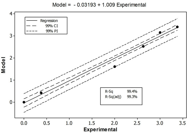
Figure 7. Regression fit analysis between experimental data and PDM, showing the prediction (PI) and confidence (CI) intervals for cumulative mercury concentration.