Existence and Uniqueness of Solutions to Impulsive Fractional Integro-Differential Equations with Nonlocal Conditions ()
1. Introduction
Fractional differential equations appear naturally in a number of fields such as physics, engineering, biophysics, blood flow phenomena, aerodynamics, electron-analytical chemistry, biology, control theory, etc., An excellent account in the study of fractional differential equations can be found in [1-11] and references therein. Undergoing abrupt changes at certain moment of times like earthquake, harvesting, shock etc, these perturbations can be well-approximated as instantaneous change of state or impulses. Furthermore, these processes are modeled by impulsive differential equations. In 1960, Milman and Myshkis introduced impulsive differential equations in their papers [12]. Based on their work, several monographs have been published by many authors like Semoilenko and Perestyuk [13], Lak-shmikantham et al. [14], Bainov and Semoinov [15,16], Bainov and Covachev [17] and Benchohra et al. [18]. Impulsive fractional differential equations represent a real framework for mathematical modelling to real world problems. Significant progress has been made in the theory of impulsive fractional differential equations [19-21].
We consider a class of impulsive fractional integrodifferential equations with nonlocal conditions of the form
 (1.1)
(1.1)
 (1.2)
(1.2)
 (1.3)
(1.3)
Where  is the Caputo fractional derivative, the function
  is continuous and the function
  is continuous,

and  represent the right and left limits of
  at
at , and
, and is a continuous function,
 .
.
Nonlocal conditions were initiated by Byszewski [22] who proved the existence and uniqueness of mild and classical solutions of nonlocal Cauchy problems. As remarked by Byszewski [23,24], the nonlocal condition can be more useful than the standard initial condition to describe some physical phenomena. For example,  may be given by
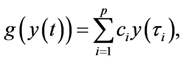
where  are given constants and
  .
.
In this article, our aim is to show sufficient conditions for the existence and uniqueness of solutions of solutions to impulsive fractional integro-differential equations with nonlocal conditions.
2. Preliminaries
In this section, we introduce some notations, definitions and preliminary facts which are used throughout this paper. By  we denote the Banach space of all continuous functions from
  into
into  with the norm
Definition 2.1 [5,8]: The fractional (arbitrary) order integral of the function  of order
  is defined by

where  is the gamma function, when
Definition 2.2 [5,8]: For a function  given on the interval
 , Riemann-Liouville fractional-order derivative of order
  of
of , is defined by

here  and
and  denotes the integer part of
 , when
 .
.
Definition 2.3 [14]: For a function  given on the interval
 , the Caputo fractional-order derivative of order
  of
of , is defined by

where .
.
Lemma 2.4 [25]: (Schaefer’s fixed point theorem). Let  be a Banach space and
  be a completely continuous operator. If the set
 is bounded, then
  has at least a fixed point in X.
3. Existence of Solutions
Consider the set of functions

Definition 3.1: A function  whose
whose  -derivative exists on
  is said to be a solution of (1.1)-(1.3), if
  satisfies the equation

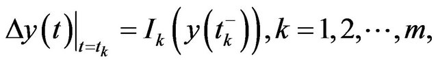
on  and satisfies the conditions

where .
.
To prove the existence of solutions to (1.1)-(1.3), we need the following auxiliary lemmas.
Lemma 3.2: Let , then the equation

has solutions

Lemma 3.3: Let , then

for some .
.
As a consequence of Lemma 3.2 and Lemma 3.3, we have the following result Lemma 3.4: Let , and let
  be continuous. A function
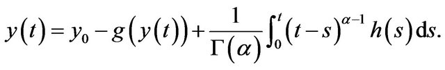
  is a solution of the fractional integral equation
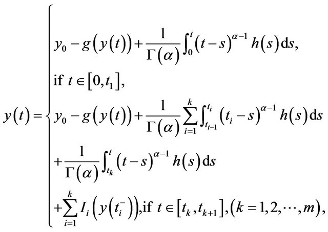 (3.1)
(3.1)
if and only if  is a solution of the fractional nonlocal BVP
 (3.2)
(3.2)
 (3.3)
(3.3)
 (3.4)
(3.4)
Proof Assume  satisfies (3.2)-(3.4).
If  then
then .
.
Lemma 3.3 implies
If , by Lemma 3.3, it follows that

If , then from Lemma 3.3 we get
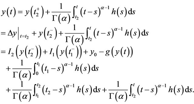
If , then again from
  we have (3.1).
Conversely, assume that  satisfies the impulsive fractional integral equation (3.1). If
 , then
  and using the fact that
  is the left inverse of
 , we get
 .
.
If  and using the fact that
 , where
  is a constant, we conclude that
Also, we can easily show that

Theorem: Assume that:
(H1) There exists a constant  such that
 for each
  and each
 ;
;
(H2) There exists a constant  such that
 , for each
  and
and ;
;
(H3) There exists a constant  such that
 , for each
 , then the problem
(1.1)-(1.3) has at least one solution on .
.
Proof Consider the operator
 defined by

Clearly, the fixed points of the operator  are solution of the problem (1.1)-(1.3).
We shall use Schaefer’s fixed point theorem to prove that  has a fixed point. The proof will be given in several steps.
Step 1:  is continuous.
Let  be a sequence such that
  in
in . Then for each
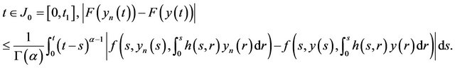
Since  is continuous function, we have
 as
as .
.
For each ,
,

Since  and
and  are continuous functions, we have
  as
as .
.
Therefore,  is continuous.
Step 2:  maps bounded sets into bounded sets in
 .
.
Indeed, it is enough to show that for any , there exists a positive constant
  such that for each
 , we have
 . By (H1), (H2) and (H3), for each
 , we have
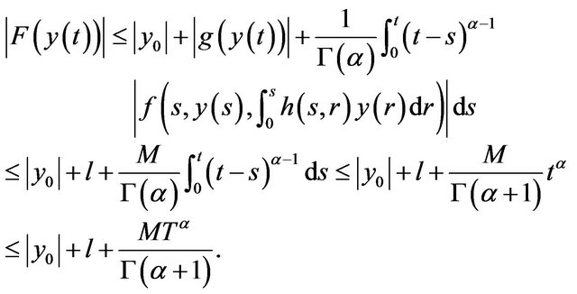
For , we have

Let
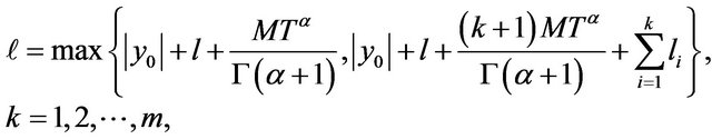
then 
Step 3:  maps bounded sets into equicontinuous sets of
 .
.
Let ,
,  be a bounded set of
  as in Step 2, and let
 . For
. For
 , we have

For , we have

As , the right-hand side of the above inequality tends to zero. As a consequence of Steps 1 to 3 together with the Arzel’a-Ascoli theorem, we can conclude that
  is completely continuous.
As a consequence of Lemma 2.4 (Schaefer’s fixed point theorem), we deduce that  has a fixed point which is a solution of the problem (1.1)-(1.3).
4. Acknowledgements
This work was supported by the natural science foundation of Hunan Province (13JJ6068, 12JJ9001), Hunan provincial science and technology department of science and tech-neology project (2012SK3117), Science foundation of Hengyang normal university of China (No. 12B35) and Construct program of the key discipline in Hunan Province.