An EOQ Model for Deteriorating Items with Linear Demand, Variable Deterioration and Partial Backlogging ()
1. Introduction
Recently, deteriorating items in inventory system have become an interesting feature for its practical importance. Generally, deterioration is defined as damage, decay or spoilage. Food items, photographic films, drugs, chemicals, pharmaceuticals, electronic components and radioactive substances are some examples of items in which sufficient deterioration may occur during the normal storage period of units and consequently the loss must be taken into account while analyzing the inventory system. Spoilage in food grain storage, decay in radioactive elements, pilferages from on-hand inventory is continuous in time. Therefore, the effect of deterioration of physical goods cannot be disregarded in many inventory systems. Ghare and Schrader [1] first derived a revised economic order quantity by assuming exponential decay. Covert and Philip [2] extended Ghare and Schrader’s constant deterioration rate to a two-parameter Weibull distribution. Later, Shah and Jaiswal [3] and Aggarwal [4] presented and re-established an order level inventory model with a constant rate of deterioration respectively. Dave and Patel [5] considered an inventory model for deteriorating items with time-proportional demand when shortages were not allowed. Later, Sachan [6] extended the model to all for shortages. Hollier and Mak [7], Hariga and Benkherouf [8], Wee [9,10] developed their models taking the exponential demand. Earlier, Goyal and Giri [11], wrote an excellent survey on the recent trends in modeling of deteriorating inventory. For the items like fruits and vegetables, whose deterioration rate increases with time. Ghare and Schrader [1] were the first to use the concept of deterioration followed by Covert and Philip [2] who formulated a model with variable rate of deterioration with two-parameter Weibull distributions, which was further extended by Philip [12] considering a variable deterioration rate of three-parameter Weibull distributions. In some inventory systems, the longer the waiting time is, the smaller the backlogging rate would be and vice versa. Therefore, during the shortage period, the backlogging rate is variable and dependent on the waiting time for the next replenishment. Chang and Dye [13] developed an EOQ model allowing shortage. Recently, Ouyang, Wu and Cheng [14] established an EOQ inventory model for deteriorating items in which demand function is exponential declining and partially backlogging.
In the present paper attempts have been made to investigate an EOQ model with deteriorating items that deteriorates according to a variable deterioration rate. Here we assumed the demand function is linear pattern and the backlogging rate is inversely proportional to the waiting time for the next replenishment. Ever till now, most of the researchers have been either completely ignoring the deterioration factor or are considering a constant rate of deterioration, which is not possible practical. Since the effect of deterioration cannot be ignored, we have taken a variable deterioration. The objective of the model is to determine the optimal order quantity and the length of the ordering cycle in order to minimize the total relevant cost. A numerical example is cited to illustrate the model and a sensitivity analysis of the optimal solution is carried out.
2. Assumptions
The following assumptions are made in developing the model.
1) The inventory system involves only one item and the planning horizon is infinite.
2) Replenishment occurs instantaneously at an infinite rate.
3) The deteriorating rate , is a variable deterioration and there is no replacement or repair of deteriorated units during the period under consideration.
4) The demand rate, 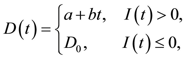 where
where
 and
and  is initial demand.
5) During the shortage period, the backlogging rate is variable and is dependent on the length of the waiting time for the next replenishment. The longer the waiting time is, the smaller the backlogging rate would be. Hence, the proportion of customers who would like to accept backlogging at time  is decreasing with the waiting time
  waiting for the next replenishment. To take care of this situation we have defined the backlogging rate to be
  when in ventory is negative. The backlogging parameter
  is a positive constant,
 .
.
3. Notations
The following notations have been used in developing the model.
1)  : holding cost, $/per unit/per unit time.
2)  : cost of the inventory item, $/per unit.
3)  : ordering cost of inventory, $/per order.
4)  : shortage cost, $/per unit/per unit time.
5)  : opportunity cost due to lost sales, $/per unit.
6)  : time at which shortages start.
7)  : length of each ordering cycle.
8)  : the maximum inventory level for each ordering cycle.
9)  : the maximum amount of demand backlogged for each ordering cycle.
10)  : the economic order quantity for each ordering cycle.
11)  : the inventory level at time
 .
.
12)  : the optimal solution of
 .
.
13)  : the optimal solution of
 .
.
14)  : the optimal economic order quantity.
15)  : the optimal maximum inventory level.
16)  : the minimum average total cost per unit time.
4. Mathematical Formulation
We consider the deteriorating inventory model with linear demand. Replenishment occurs at time  when the inventory level attains its maximum,
 . From
  to
to , the inventory level reduces due to demand and deterioration. At time
 , the inventory level achieves zero, then shortage is allowed to occur during the time interval
  and all of the demand during shortage period
  is partially backlogged.
As the inventory level reduces due to demand rate as well as deterioration during the inventory interval , the differential equation representing the inventory status is governed by
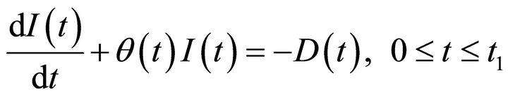 , (1)
, (1)
where  and
and .
.
The solution of Equation (1) using the condition  is
is
 .(2)
.(2)
(neglecting the higher power of  as
as ).
).
Maximum inventory level for each cycle is obtained by putting the boundary condition  in Equation (2). Therefore,
 . (3)
. (3)
During the shortage interval , the demand at time
  is partially backlogged at the fraction
 . Therefore, the differential equation governing the amount of demand backlogged is
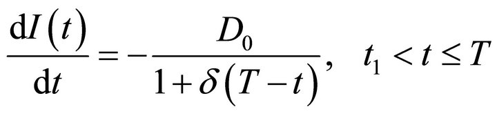 . (4)
. (4)
with the boundary condition .
.
The solution of Equation (4) is
 . (5)
. (5)
Maximum amount of demand backlogged per cycle is obtained by putting  in Equation (5). Therefore,
 . (6)
. (6)
Hence, the economic order quantity per cycle is
 . (7)
. (7)
The inventory holding cost per cycle is
 . (8)
. (8)
(neglecting the higher power of  as
as ).
).
The deterioration cost per cycle is
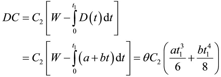 . (9)
. (9)
The shortage cost per cycle is
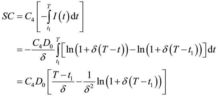 . (10)
The opportunity cost due to lost sales per cycle is
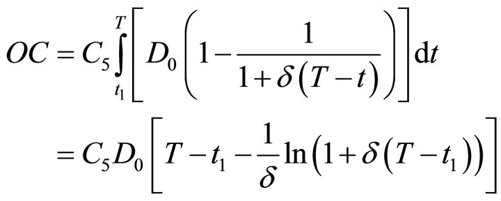 . (11)
Therefore, the average total cost per unit time per cycle = (holding cost + deterioration cost + ordering cost + shortage cost + opportunity cost due to lost sales)/length of the ordering cycle, i.e.,
 . (12)
Our aim is to determine the optimal values of  and
and  in order to minimize the average total cost per unit time,
 .
.
Using calculus, we now minimize . The optimum values of
  and
and  for the minimum average cost
  are the solutions of the equations
 and
and , (13)
provided that they satisfy the sufficient conditions
 ,
,  and
and
 .
.
Equation (13) can be written as
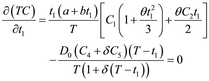 . (14)
and
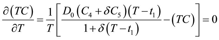 . (15)
Now,  and
and  are obtained from the Equations (13) and (14) respectively. Next, by using
  and
and , we can obtained the optimal economic order quantity, the optimal maximum inventory level and the minimum average total cost per unit time from Equations (7), (3) and (12) respectively.
5. Numerical Example
In this section, we provide a numerical example to illustrate the above theory.
Example 1: Let us take the parameter values of the inventory system as follows:
 ,
,  ,
,  ,
,  ,
,  ,
,  ,
,  ,
,  ,
,  , and
, and .
.
Solving Equations (14) and (15), we have the optimal shortage period  unit time and the optimal length of ordering cycle
  unit time. Thereafter, we get the optimal order quantity
  units, the optimal maximum inventory level
  units and the minimum average total cost per unit time
 .
.
6. Sensitivity Analysis
We study now study the effects of changes in the values of the system parameters ,
,  ,
,  ,
,  ,
,  ,
,  ,
,  ,
,  ,
,  and
and  on the optimal total cost and number of reorder. The sensitivity analysis is performed by changing each of parameters by +50%, +10%, −10% and −50% taking one parameter at a time and keeping the remaining parameters unchanged.
The analysis is based on the Example 1 and the results are shown in Table 1. The following points are observed.
1)  &
&  decrease while
  increases with the increase in value of the parameter
 . Both
  &
&  are highly sensitivity to change in
  and
and  is moderately sensitive to change in
 .
.
2)  &
&  decrease while
  increases with the increase in value of the parameter
 . Both
  &
&  are moderately sensitive to change in
  and
and  is low sensitive to change in
 .
.
3)  &
&  decrease while
  increases with the increase in value of the parameter
 . Here
  &
&  and
and  are highly sensitive to change in
 .
.
4)  &
&  decrease while
  increases with the increase in value of the parameter
 . Here
 ,
,  and
and  are low sensitive to change in
 .
.
5)  ,
,  &
&  increase with the increase in value of the parameter
 . Here
 ,
,  and
and  are highly sensitive to change in
 .
.
6)  &
&  increase while
  decreases with the increase in value of the parameter
 . Here
  &
&  and
and  are moderately sensitive to change in
 .
.
7)  &
&  increase while
  decreases with the increase in value of the parameter
 . Here
 ,
,  and
and  are moderately sensitive to change in
 .
.
8)  &
&  increase while
  decreases with the increase in value of the parameter
 . Here
 ,
,  and
and  are moderately sensitive to change in
 .
.
9)  &
&  decrease while
  increases with the increase in value of the parameter
 . Here
 ,
,  and
and  are low sensitive to change in
 .
.
10)  &
&  increase while
  decreases with the increase in value of the parameter
 . Here
 ,
,  and
and  are moderately sensitive to change in
 .
.
7. Conclusions
The economic order quantity (EOQ) model considered above is suited for items having variable deterioration rate, earlier models have considered items having constant rate of deterioration. This model can be used for items like fruits and vegetables whose deterioration rate increase with time. Demand pattern considered here is linear demand patterns and the backlogging rate is inversely proportional to the waiting time for the next replenishment. Furthermore, we have used the numerical example by minimizing the total cost by simultaneously optimizing the shortage period and the length of cycle. Finally, we have studied the sensitivity analysis of the various parameters on the effect of the optimal solution.
While this research provides the better solution, further investigation can be conducted in a number of directions. For instance, we may extend the proposal model to allow for different deterministic demand (constant, quadratic, power and others). Also, we could consider the effects of the variable deteriorations (two-parameter Weibull, three-parameter Weibull and Gamma distribution). Finally, we could generalize the model to stochastic fluctuating demand patterns and the economic production lot size model.
8. Acknowledgements
The authors would like to thank the referee for helpful comments.