Multigrid Method for the Numerical Solution of the Modified Equal Width Wave Equation ()
Received 3 April 2016; accepted 21 June 2016; published 24 June 2016

1. Introduction
A large system of equations comes out from discretization of the domain of partial differential equations into a collection of points and the optimal method for solving these problems is multigrid method, see [1] - [4] .
The modified equal width wave (MEW) equation introduced by Morrison et al. [5] is used as a model equation to describe the nonlinear dispersive waves. Gardner and Gardner [6] [7] solved the EW equation with the Galerkin’s method using cubic B-splines as a trial and test function. The MEW equation was similar with the modified regularized long wave (MRLW) equation [8] and modified Korteweg-de Vries (MKdV) equation [9] . All the modified equations are nonlinear wave equations with cubic nonlinearities and all of them have solitary wave solutions, which are wave packets or pulses. These waves propagate in non-linear media by keeping wave forms and velocity even after interaction occurs.
Several solutions for MEW had been proposed in [10] - [22] . In Geyikli and Battal Gazi Karakoc [10] [11] , the solutions are based on septic B-spline finite elements and Petrov-Galerkin finite element method with weight functions quadratic and element shape functions which are cubic B-splines. Esen [12] [13] solved the MEW equation by applying a lumped Galerkin method based on quadratic B-spline finite elements. Saka [14] proposed algorithms for the numerical solution of the MEW equation using quintic B-spline collocation method. Zaki [15] considered the solitary wave interactions for the MEW equation by collocation method using quintic B-spline finite elements and obtained the numerical solution of the EW equation by using least-squares method [16] . Wazwaz [17] investigated the MEW equation and two of its variants by the tanh and the sine-cosine methods. A solution based on a collocation method incorporated cubic B-splines is investigated by Saka and Dağ [18] . Lu [19] presented a variational iteration method to solve the MEW equation. Evans and Raslan [20] studied the generalized EW equation by using collocation method based on quadratic B-splines to obtain the numerical solutions of a single solitary waves and the birth of solitons. Esen and Kutluay [21] studied a linearized implicit finite difference method in solving the MEW equation. Battal Gazi Karakoc and Geyikli [22] solved the MEW equation by a lumped Galerkin method using cubic B-spline finite elements.
An outline of this paper is as follows: We begin in Section 2 by reviewing the analytical solution of the MEW equation. In Section 3, we derive a new numerical method based on the multigrid technique and finite difference method for obtaining the numerical solution of MEW equation. Finally, in Section 4, we introduce the numerical results for solving the MEW equation through some well known standard problems.
2. The Analytical Solution
The modified equal width wave equation which is as a model for non-linear dispersive waves, considered here has the normalized form [5]
 (1)
(1)
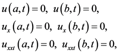
with the physical boundary conditions  as
as , where t is time and x is the space coordinate,
  is a positive parameter. For this study boundary conditions are chosen
 (2)
(2)
and the initial condition as

where f is a localized disturbance inside the considered interval.
The exact solution of equation (1) can be written in the form [15]
 (3)
(3)
which represents the motion of a single solitary wave with amplitude A, where the wave velocity  and
and . The initial condition is given by
 (4)
(4)
For the MEW equation, it is important to discuss the following three invariant conditions given in [15] , which, respectively, correspond to conversation of mass, momentum, and energy. The analytical values of the invariants are
 (5)
(5)
3. Numerical Method
The basic idea of multigrid techniques is illustrated by Brandt [1] . In this section we apply this method for initial boundary value problem, except that, the upper boundary conditions change with time, in which the initial condition is  for
for . Dividing the interval of time to K parts, we obtain the solutions of the partial differential equation at time t1 and use these solutions as initial values for the next level
 , and for the other, we obtain the solutions at time T. The numbers of points in a coarse grid for this domain are two points.
We apply the full multigrid algorithm for the MRLW equation. Assuming the initial condition ![]() and the solution
and the solution![]() ,
, ![]() has the usual partition with a space step size
has the usual partition with a space step size ![]() and a time step size
and a time step size ![]() (
(![]() ).
).
We start handling the non-linear term ![]() by expressing in the form
by expressing in the form![]() . The back-time and centre-
. The back-time and centre-
space difference for Equation (1) is
![]() (6)
(6)
where![]() ,
, ![]() for a set grids
for a set grids ![]()
Step 1: ![]()
Step 2: Starting from ![]() in the coarse grid, we can calculate the approximate value
in the coarse grid, we can calculate the approximate value ![]() at two points using Equation (5) leading to:
at two points using Equation (5) leading to:
![]() (7)
(7)
The right hand side for equation (7) can be computed using the initial and boundary conditions.
Step 3: Interpolating the grid functions from the coarse grid to fine grid using linear interpolation![]() , in which
, in which
![]() (8)
(8)
that can be written explicitly as:
![]() (9)
(9)
Step 4: Doing relaxation sweep on ![]() using the point relaxation
using the point relaxation
![]() (10)
(10)
Step 5: Computing the residuals ![]() on
on ![]() and inject them into
and inject them into ![]() using full weighting restriction
using full weighting restriction ![]() to get
to get ![]() as:
as:
![]() (11)
(11)
![]() (12)
(12)
Step 6: Computing an approximate solution of error![]() .
.
Step 7: Interpolating the solution of error ![]() onto
onto![]() ,
, ![]() and adding it to
and adding it to ![]() which is the approximate value of u on the fine grid with
which is the approximate value of u on the fine grid with![]() .
.
By taking this solution on coarse grid and repeating steps 3-7, we obtain the approximate values of u on the grid with ![]() and so
and so ![]() the final value is the solution at the time level
the final value is the solution at the time level![]() .
.
Step 8:![]() , go to step 2 (lead to the solution at higher time level as needed).
, go to step 2 (lead to the solution at higher time level as needed).
4. Numerical Results
In this section, numerical solutions of MRLW equation are obtained for standard problems as: the motion of single solitary wave, interaction of two solitary waves and development of Maxwellian initial condition into solitary waves. For the MEW equation, it is important to discuss the following three invariant conditions given in [15] , which respectively correspond to conversation of mass, momentum and energy:
![]() (13)
(13)
The accuracy of the method is measured by both the ![]() error norm
error norm
![]() (14)
(14)
and the ![]() error norm
error norm
![]() (15)
(15)
to show how good the numerical results in comparison with the exact results.
4.1. The Motion of Single Solitary Wave
Consider Equation (1) with boundary conditions (2) and the initial condition (4). For a comparison with earlier studies [13] [19] [21] [22] we take the parameters ![]() and
and ![]() over the interval [0, 80]. To find the error norms
over the interval [0, 80]. To find the error norms![]() ,
, ![]() and the numerical invariants
and the numerical invariants ![]() and
and ![]() at various times we use the numerical solutions by applying the multigrid method up to
at various times we use the numerical solutions by applying the multigrid method up to![]() . As reported in Table 1, the error norms
. As reported in Table 1, the error norms![]() ,
, ![]() are found to be small enough, and the computed values of invariants are in good agreement with their analytical values
are found to be small enough, and the computed values of invariants are in good agreement with their analytical values ![]() Table 2 shows a comparison of the values of the invariants and error norms obtained by the present method with those obtained by other methods [13] [19] [21] [22] . It is clearly seen from Table 2 that the error norms obtained by the present method are smaller than the other methods.
Table 2 shows a comparison of the values of the invariants and error norms obtained by the present method with those obtained by other methods [13] [19] [21] [22] . It is clearly seen from Table 2 that the error norms obtained by the present method are smaller than the other methods.
4.2. Interaction of Two Solitary Waves
Consider the interaction of two positive solitary waves as a second problem. For this problem, the initial condition is given by:
![]() (16)
(16)
For the computational discussion, firstly we use parameters ![]()
![]() and
and ![]() over the range
over the range ![]() to coincide with those used in [22] .
to coincide with those used in [22] .
In [20] the analytic invariants are![]() ,
, ![]() ,
,![]() . The experiment is run from
. The experiment is run from ![]() to
to ![]() and values of the invariant quantities
and values of the invariant quantities ![]() and
and ![]() are listed in Table 3.
are listed in Table 3.
Table 3 shows a comparison of the values of the invariants obtained by present method with those obtained in
![]()
Table 1. Invariants and error norms for single solitary wave when![]() .
.
![]()
Table 2. Comparison of errors and invariants for single solitary wave at![]() .
.
![]()
Table 3. Comparison of invariants for the interaction of two solitary waves with results from [22] (![]()
![]() ).
).
[22] . It is seen that the numerical values of the invariants remain almost constant during the computer run.
Finally, we have studied the interaction of two solitary waves with the following parameters ![]()
![]() and
and ![]() in the range [0,150].
in the range [0,150].
The analytical invariants can be found as in [22] ![]() ,
, ![]() ,
,![]() . The experiment is run from t = 0 to t = 55 and values of the invariant quantities
. The experiment is run from t = 0 to t = 55 and values of the invariant quantities ![]() and
and ![]() are listed in Table 4.
are listed in Table 4.
4.3. The Maxwellian Initial Condition
Last study, we consider the numerical solution of the equation (1) with the Maxwellian initial condition
![]() (17)
(17)
and the boundary conditions ![]()
![]()
Table 4. Invariants for the interaction of two solitary waves (![]() ).
).
![]()
Table 5. Invariants of MEW equation using the Maxwelliancondition![]() .
.
It is known that the behavior of the solution with the Maxwellian condition (17) depends on the values of![]() . So we have considered various values for
. So we have considered various values for![]() . The computations are carried out for the cases
. The computations are carried out for the cases ![]()
![]() and 0.005 which are used in the earlier papers [15] [19] . The numerical conserved quantities with
and 0.005 which are used in the earlier papers [15] [19] . The numerical conserved quantities with ![]() and 0.005 are given in Table 5. It is observed that the obtained values of the invariants remain almost constant during the computer run.
and 0.005 are given in Table 5. It is observed that the obtained values of the invariants remain almost constant during the computer run.
5. Conclusion
In this paper we study the MEW problem by extending the use of multigrid technique. We checked our scheme through single solitary wave in which the analytic solution is known. Our scheme was extended to study the interaction of two solitary waves and Maxwellian initial condition where the analytic solutions are unknown during the interaction. The performance and accuracy of the method were explained by calculating the error norms ![]() and conservative properties of mass, momentum and energy. The computed results showed that our scheme is a successful numerical technique for solving the MEW problem and can be also efficiently applied for solving a large number of physically important non-linear problems.
and conservative properties of mass, momentum and energy. The computed results showed that our scheme is a successful numerical technique for solving the MEW problem and can be also efficiently applied for solving a large number of physically important non-linear problems.